REVIEW 4 major objections 3 minor 57 references
Imaging Anisotropic Conductivity from Internal Measurements with Mixed Least-Squares Deep Neural Networks
T0 review · 4 major / 3 minor · reviewed 2026-08-12 · deepseek-v4-flash
Pith's one-line read The paper develops a mixed least-squares deep neural network that approximates the internal flux and the anisotropic conductivity tensor simultaneously from internal measurements of the solution, and proves error bounds of order…
desk verdict Solid anisotropic extension of the MLS-DNN method with convincing numerics, but the proof of the main error bound has a real gap and the theory only covers global minimizers, so the theorem is unproven as written. read the letter →
The pith
A machine-rendered reading of the paper's core claim, the machinery that carries it, and where it could break.
The reading
What carries the argument
The load-bearing object is the mixed least-squares loss built from the first-order system $\sigma_i=A\nabla u_i$, $-\nabla\cdot\sigma_i=f_i$, with the relevant boundary condition, so that the conductivity and the flux are both unknowns fitted to the internal measurements. The loss uses a matrix-valued projection $P_K$, applied pointwise by eigenvalue decomposition and clipping eigenvalues to $[c_0,c_1]$, to keep $A_\theta$ inside the admissible set of uniformly elliptic symmetric matrices; the projection also enters the error analysis through the variational inequality that characterizes it. The convergence proof combines three tools: DNN approximation rates for $\tanh$ networks (giving the representation errors $\epsilon_A,\epsilon_\sigma$), the projected source condition $A^\dagger=P_K(\nabla u^\dagger\otimes\nabla\psi)$ that turns the $L^2$ error into computable residuals, and Rademacher-complexity bounds for the Monte Carlo empirical loss.
What would settle it
Choose a smooth full anisotropic tensor $A^\dagger$ that does not satisfy the projected source condition $A^\dagger=P_K(\nabla u^\dagger\otimes\nabla\psi)$ and run the MLS-DNN with exact data, taking $\gamma_A\to 0$ and large DNN capacity. If the empirical $L^2$ error $e(\hat A)$ stops decreasing at a positive plateau rather than following the predicted $O(\delta^{1/2})$ rate, the bound's premise --- a global minimizer plus the source condition --- is not what governs the reported accuracy.
Extended reading notes
Core claim
The central claim is that the mixed least-squares deep neural network recovers the anisotropic conductivity tensor $A^\dagger$ by minimizing the loss $J_\gamma(\theta,\kappa) = \sum_i(\|\sigma_{i,\kappa}-P_K(A_\theta)\nabla z_i^\delta\|^2_{L^2(\Omega)^d} + \gamma_\sigma\|\nabla\cdot\sigma_{i,\kappa}+f_i\|^2_{L^2(\Omega)} + \gamma_b\|n\cdot\sigma_{i,\kappa}-g_i\|^2_{L^2(\partial\Omega)} + \gamma_A\|P_K(A_\theta)\|^2_{L^2(\Omega)^{d,d}})$ for the Neumann problem, with a Dirichlet analogue, where $P_K$ is the orthogonal projection onto the admissible set of uniformly elliptic symmetric matrices. Theorem 3.1 gives $\|A^\dagger - P_K(A^*_\theta)\|_{L^2(\Omega)^{d,d}} \le c(\gamma_A^{-1}\eta^2+\eta+(1+\gamma_\sigma^{-1}+\gamma_b^{-1})\gamma_A)^{1/2}$ with $\eta$ combining DNN approximation error, noise level $\delta$, and the penalties, and Theorem 3.2 extends the bound to the empirical loss with Monte Carlo quadrature error terms. With the parameter choice $\gamma_A\sim\delta$, $\epsilon_A=\epsilon_\sigma\sim\delta$, the rate is $O(\delta^{1/2})$, comparable to output least-squares Galerkin methods. The experiments demonstrate reconstruction of full matrix-valued conductivities in 2D and 3D with data noise up to 10 percent, including from partial internal data.
Load-bearing premise
The error bounds apply only to an exact global minimizer of the nonconvex training loss, but the actual computations use a gradient optimizer that may stop at a local minimum; the paper states that optimization errors can be pronounced and that for exact data the reconstruction cannot be made arbitrarily accurate.
Editorial extensions
If this is right
- An anisotropic conductivity tensor in 2D and 3D can be reconstructed from internal solution measurements without labeled training pairs, using an unsupervised DNN that fits flux and conductivity simultaneously.
- With $\gamma_A\sim\delta$ and representation errors of order $\delta$, the reconstruction error in $L^2(\Omega)^{d,d}$ is of order $\delta^{1/2}$, the same rate as classical output least-squares Galerkin methods.
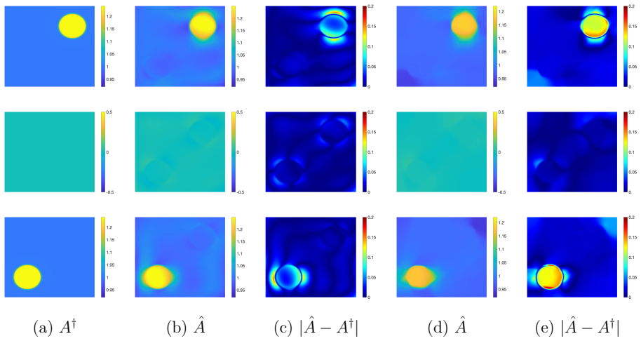
- The method handles partial internal data: reconstructions remain accurate over the whole domain even when measurements are confined to a boundary band, where the paper's FEM comparison shows poor stability.
- The mesh-free DNN formulation makes 3D implementation nearly identical to 2D, and the paper demonstrates 3D anisotropic reconstructions at 5 percent noise.
- For both Neumann and Dirichlet problems, the reconstruction degrades only mildly at 10 percent noise, while the PINN variant requires boundary knowledge $A^\dagger|_{\partial\Omega}$ and second-order derivatives.
Reading between the lines
- A testable extension would run the same scheme on conductivities that violate the projected source condition; the theory makes no prediction for them, so a numerical rate study would show whether the method's practical accuracy outruns the proved bound.
- The reported insensitivity to the penalty parameter $\gamma_A$ suggests the DNN's implicit spectral bias is doing regularization work that the analysis assigns to the explicit $L^2$ penalty; separating these effects would require measuring the loss gap between the found local minimizer and the global one.
- The same mixed least-squares structure could be adapted to power-density data $A\nabla u_i\cdot\nabla u_j$ or to time-harmonic problems, where internal data are phase-sensitive; the projected source condition would need re-derivation for those settings.
Editorial analysis
A structured set of objections, weighed in public.
Referee Report
Summary. The paper develops a deep-learning approach (MLS-DNN) for recovering an anisotropic conductivity tensor A from internal measurements of solutions to an elliptic boundary value problem. The method is based on a mixed least-squares formulation in which the flux sigma and the conductivity A are represented by tanh neural networks, with the constraint A in K enforced by a matrix-valued projection. The authors prove error estimates for the L2 reconstruction error of the projected DNN conductivity for global minimizers of both the population loss (Theorem 3.1) and the empirical loss (Theorem 3.2), assuming a projected source condition, DNN approximation rates, and Rademacher-type statistical bounds. They also present numerical experiments for Neumann and Dirichlet problems in 2D and 3D, with full or partial data and up to 10% noise, comparing with FEM and PINN.
Significance. If the theoretical results were fully rigorous and connected to the implemented algorithm, the paper would offer an important extension of the Kohn-Lowe mixed formulation and of the isotropic MLS-DNN framework to anisotropic problems, with the first numerical demonstrations in 3D. The numerical study is genuinely useful: it shows stable recovery for several nontrivial anisotropic examples, including partial interior data, and the authors state that code will be released. The main caveats are that the error bounds apply only to exact global minimizers, which the ADAM-trained networks need not be, and that one step in the proof of Theorem 3.1 rests on an equality that is not implied by the source condition. These issues limit the theoretical support for the headline claim of accurate recovery up to 10% noise, although the empirical evidence stands independently.
major comments (4)
- [Section 3.1, proof of Theorem 3.1] The displayed equality (A†, A†−PK(A*θ)) = ((A†−PK(A*θ))∇u†, ∇ψ) is not an identity under Assumption 3.2; the assumption gives A† = PK(∇u†⊗∇ψ), not A† = ∇u†⊗∇ψ. From the projection inequality (2.4) one only obtains the inequality (A†, A†−PK(A*θ)) ≤ ((A†−PK(A*θ))∇u†, ∇ψ). Since the subsequent argument bounds the absolute value, replacing the equality by this inequality appears to repair the proof, but the current text contains a false equality and should be corrected.
- [Section 3 (Theorems 3.1 and 3.2) and Section 4] The theorems bound the reconstruction error of global minimizers of the population and empirical losses, but the reported reconstructions are obtained by ADAM on the nonconvex empirical loss. The paper itself states in Section 4 that 'the optimizer may get trapped in a local minimum, leading to pronounced optimization errors' and that for exact data 'the reconstruction cannot be made arbitrarily accurate.' Consequently, the O(δ^{1/2}) error bound is not established for the computed solutions, and the numerical results do not verify the theorem quantitatively. The authors should either add an optimization-error estimate or an explicit condition under which the ADAM solution is close to a global minimizer, or clearly separate the theoretical claim (for global minimizers) from the numerical demonstration (which is then purely empirical).
- [Section 4, noise generation] The theoretical noise model in (2.3) and (2.11) measures δ = ∥u† − zδ∥ in H^1(Ω) or H^{3/2}(Ω), while the experiments add i.i.d. Gaussian noise pointwise to ∇u† (Section 4: 'i.i.d. Gaussian noise is added pointwise to ∇u†'). A pointwise-perturbed gradient is generally not in H^1(Ω), so the experimental data do not satisfy the regularity assumptions of Theorem 3.2. If the noisy gradient is meant to be a smoothed version of raw data, the smoothing procedure and its effect on δ should be described; otherwise the numerical experiments do not directly test the noise-dependence predicted by the theory.
- [Lemma 3.2] Lemma 3.2 is central to the empirical-loss bound, but its proof is omitted and is referred to [30, Theorem 3.4]. The loss here involves the anisotropic projection PK(Aθ) and additional boundary terms, so it is not immediately obvious that the argument transfers verbatim. A proof or a precise statement of the required changes should be included, rather than delegating to the authors' previous paper.
minor comments (3)
- [Section 2.2, after (2.5)] The tuple γ is defined as (γσ, γb, γq) ∈ R^3_+, but γq never appears; the third component should be γA.
- [Section 4, paragraph after Table 1] The sentence 'This strategy is often used for tuning hyper-parameters in deep learning' refers to choosing hyperparameters that attain the smallest reconstruction error on the test examples; this selection procedure should be stated in the abstract or conclusions if the claimed accuracy is based on it.
- [Throughout] There are several typos: 'b e tween' after (2.4), 'reonstruction' in Table 2 heading, 'off-shelf' in Section 4, and 'Combing' in the proof of Theorem 3.1. These should be corrected.
Circularity Check
No circular reduction in the central error analysis; one technical lemma is deferred to the authors' prior work, but no fitted parameter is disguised as a prediction.
full rationale
The central derivation is not circular. The reconstruction is obtained by minimizing the mixed least-squares losses (2.5)/(2.7) or (2.12)/(2.13) over DNN parameters, and Theorems 3.1 and 3.2 bound the distance between A† and the projected DNN reconstruction in terms of the noise level δ, DNN approximation errors ϵA, ϵσ, and Monte Carlo sampling errors. Assumption 3.2, A† = P_K(∇u†⊗∇ψ), is a structural source condition on the unknown conductivity rather than a restatement of the algorithm's output; it controls one inner-product term in the proof, and the final bound still depends on the actual loss residuals. No fitted parameter is renamed as a prediction: the hyperparameters in Section 4 are tuned to minimize the reported benchmark error, but this is a standard experimental evaluation against known exact solutions, not a derivation of the theoretical rate. The only self-referential element is Lemma 3.2, whose proof is omitted with the sentence 'The proof follows identically as that of [30, Theorem 3.4]'; reference [30] shares three authors with this paper. This is reliance on a self-citation for a Rademacher-complexity quadrature bound, but that bound is a separate statistical-learning estimate and is not equivalent to the target conductivity-recovery result, so it does not make the central claim circular. Two non-circular limitations are explicitly flagged here and weighed in the verdict: the theorems apply to exact global minimizers of nonconvex losses, while ADAM may return a local minimum (Section 4 concedes that 'the optimizer may get trapped in a local minimum'), and the experiments add noise to ∇u† while the theory measures δ = ∥u†-zδ∥_{H1}; these are gaps between theory and numerics, not circularity.
Assumptions & free parameters
free parameters (5)
- Regularization weight γA =
1e-5 (all experiments, Table 1)
- Divergence and boundary penalty weights γσ, γb =
e.g., (1,1) for noise-free, (10,2.5) for noisy in Examples 4.1/4.2; different values in other examples (Table 1)
- Early stopping epoch =
e.g., 8e4 for exact data, 1e4 for 10% noise in Example 4.1 (Table 1)
- DNN depth and width (LA, WA, Lσ, Wσ) =
LA=10, WA=32 for A; Lσ=5, Wσ=26 for σ; LA=5 for Examples 4.1 and 4.7
- Total variation penalty γtv =
1e-4 and 3e-3 for Example 4.4 exact/noisy; 8e-4 and 5e-3 for Example 4.10 exact/noisy
assumptions (6)
- domain assumption Assumption 3.1: A† ∈ W^{2,∞}(Ω)^{d×d} ∩ K, f ∈ H^1(Ω), g ∈ H^{3/2}(∂Ω) (Neumann) or H^{5/2}(∂Ω) (Dirichlet).
- domain assumption Assumption 3.2 (projected source condition): A†(x) = P_K(∇u†(x) ⊗ ∇ψ(x)) for some ψ ∈ H^1_0(Ω) ∩ W^{2,∞}(Ω).
- domain assumption Assumption 3.3: f ∈ L∞(Ω), g ∈ L∞(∂Ω), zδ ∈ W^{1,∞}(Ω) (and on boundary in Dirichlet).
- standard math Lemma 2.1 (DNN approximation rates in Sobolev spaces), cited from [19].
- standard math Lemma 3.2 (Monte Carlo quadrature error bounds) is quoted from [30, Theorem 3.4] without proof.
- standard math Well-posedness of (1.1) and elliptic regularity, e.g., [35, Lemma 2.1] and [18].
Cite this review
Pith. "Pith review of Imaging Anisotropic Conductivity from Internal Measurements with Mixed Least-Squares Deep Neural Networks." pith.science (2026). https://pith.science/paper/2GGQK6HD
@misc{pith2026241200527,
  author       = {Pith},
  title        = {Pith review of: Imaging Anisotropic Conductivity from Internal Measurements with Mixed Least-Squares Deep Neural Networks},
  year         = {2026},
  howpublished = {\url{https://pith.science/paper/2GGQK6HD}},
  note         = {Machine review of arXiv:2412.00527}
}
read the original abstract
In this work we develop a novel algorithm, termed as mixed least-squares deep neural network (MLS-DNN), to recover an anisotropic conductivity tensor from the internal measurements of the solutions. It is based on applying the least-squares formulation to the mixed form of the elliptic problem, and approximating the internal flux and conductivity tensor simultaneously using deep neural networks. We provide error bounds on the approximations obtained via both population and empirical losses. The analysis relies on the canonical source condition, approximation theory of deep neural networks and statistical learning theory. We also present multiple numerical experiments to illustrate the performance of the method, and conduct a comparative study with the standard Galerkin finite element method and physics informed neural network. The results indicate that the method can accurately recover the anisotropic conductivity in both two- and three-dimensional cases, up to 10\% noise in the data.
Figures


Figures from the paper (15 more)




Reference graph
Works this paper leans on
-
[30]
B. Jin, X. Li, Q. Quan, and Z. Zhou. Conductivity imaging from internal measurements with mixed least-squares deep neural networks. SIAM J. Imaging Sci. , 17(1):147–187, 2024
work page 2024
-
[1]
G. Alessandrini. An identification problem for an elliptic equation in two variables. Ann. Mat. Pura Appl. (4) , 145:265–295, 1986
work page 1986
- [2]
- [3]
-
[4]
M. Anthony and P. L. Bartlett. Neural Network Learning: Theoretical Foundations . Cambridge University Press, Cambridge, 1999
work page 1999
-
[5]
G. Bal, C. Guo, and F. Monard. Imaging of anisotropic conductivities from current densities in two dimensions. SIAM J. Imaging Sci. , 7(4):2538–2557, 2014
work page 2014
-
[6]
G. Bal, C. Guo, and F. Monard. Inverse anisotropic conductivity from internal current densities. Inverse Problems, 30(2):025001, 2014
work page 2014
- [7]
Show all 57 references
-
[8]
P. L. Bartlett and S. Mendelson. Rademacher and Gaussian complexities: risk bounds and structural results. J. Mach. Learn. Res. , 3:463–482, 2002
2002
-
[9]
J. D. Bronzino and D. R. Peterson. The electrical conductivity of tissues. In Biomedical Engineering Fundamentals, pages 361–374. CRC Press, 2006
2006
-
[10]
R. H. Byrd, P. Lu, J. Nocedal, and C. Y. Zhu. A limited memory algorithm for bound constrained optimization. SIAM J. Sci. Comput. , 16(5):1190–1208, 1995
1995
-
[11]
S. Cen, B. Jin, Q. Quan, and Z. Zhou. Hybrid neural-network FEM approximation of dif- fusion coefficient in elliptic and parabolic problems. IMA J. Numer. Anal. , 44(5):3059– 3093, 2024
2024
-
[12]
S. Cen, B. Jin, K. Shin, and Z. Zhou. Electrical impedance tomography with deep Calder´ on method.J. Comput. Phys. , 493:112427, 14, 2023
2023
-
[13]
K. Chen, C. Wang, and H. Yang. Let data talk: data-regularized operator learning theory for inverse problems. Preprint, arXiv:2310.09854, 2023
2023 arXiv
-
[14]
Deckelnick and M
K. Deckelnick and M. Hinze. Convergence and error analysis of a numerical method for the identification of matrix parameters in elliptic PDEs. Inverse Problems , 28(11):115015, 15, 2012
2012
-
[15]
Dolean, A
V. Dolean, A. Heinlein, S. Mishra, and B. Moseley. Multilevel domain decomposition- based architectures for physics-informed neural networks.Comput. Methods Appl. Mech. Eng., 429:117116, 2024. 36
2024
-
[16]
W. E, J. Han, and A. Jentzen. Algorithms for solving high dimensional PDEs: from nonlinear Monte Carlo to machine learning. Nonlinearity, 35(1):278–310, 2022
2022
-
[17]
W. E and B. Yu. The deep Ritz method: a deep learning-based numerical algorithm for solving variational problems. Commun. Math. Stat. , 6(1):1–12, 2018
2018
-
[18]
Grisvard
P. Grisvard. Elliptic Problems in Nonsmooth Domains . SIAM, Philadelphia, PA, 2011
2011
-
[19]
G¨ uhring and M
I. G¨ uhring and M. Raslan. Approximation rates for neural networks with encodable weights in smoothness spaces. Neural Networks, 134:107–130, 2021
2021
-
[20]
Guo and J
R. Guo and J. Jiang. Construct deep neural networks based on direct sampling methods for solving electrical impedance tomography. SIAM J. Sci. Comput. , 43(3):B678–B711, 2021
2021
-
[21]
S. J. Hamilton and A. Hauptmann. Deep D-bar: Real-time electrical impedance tomog- raphy imaging with deep neural networks. IEEE Trans. Med. Imag., 37(10):2367–2377, 2018
2018
-
[22]
F. Hecht. New development in FreeFEM++. J. Numer. Math. , 20(3-4):251–265, 2012
2012
-
[23]
Hoell, A
N. Hoell, A. Moradifam, and A. Nachman. Current density impedance imaging of an anisotropic conductivity in a known conformal class. SIAM J. Math. Anal. , 46(3):1820– 1842, 2014
2014
-
[24]
K. H. Hoffmann and J. Sprekels. On the identification of coefficients of elliptic problems by asymptotic regularization. Numer. Funct. Anal. Optim. , 7(2-3):157–177, 1985
1985
-
[25]
G. C. Hsiao and J. Sprekels. A stability result for distributed parameter identification in bilinear systems. Math. Meth. Appl. Sci. , 10(4):447–456, 1988
1988
-
[26]
Jacot, F
A. Jacot, F. Gabriel, and C. Hongler. Neural tangent kernel: convergence and gener- alization in neural networks. In Proceedings of the 32nd International Conference on Neural Information Processing Systems , pages 8580–8589, 2018
2018
-
[27]
A. D. Jagtap, Z. Mao, N. Adams, and G. E. Karniadakis. Physics-informed neural networks for inverse problems in supersonic flows. J. Comput. Phys. , 466:111402, 18, 2022
2022
-
[28]
Y. Jiao, Y. Lai, Y. Lo, Y. Wang, and Y. Yang. Error analysis of deep Ritz methods for elliptic equations. Anal. Appl., 22(1):57–87, 2024
2024
-
[29]
B. Jin, X. Li, and X. Lu. Imaging conductivity from current density magnitude using neural networks. Inverse Problems, 38(7):075003, 36, 2022. 37
2022
-
[31]
Khoo and L
Y. Khoo and L. Ying. SwitchNet: a neural network model for forward and inverse scattering problems. SIAM J. Sci. Comput. , 41(5):A3182–A3201, 2019
2019
-
[32]
D. P. Kingma and J. Ba. Adam: A method for stochastic optimization. In 3rd Inter- national Conference for Learning Representations , San Diego, 2015
2015
-
[33]
R. V. Kohn and B. D. Lowe. A variational method for parameter identification. RAIRO Mod´ el. Math. Anal. Num´ er., 22(1):119–158, 1988
1988
-
[34]
Krishnapriyan, A
A. Krishnapriyan, A. Gholami, S. Zhe, R. Kirby, and M. W. Mahoney. Characteriz- ing possible failure modes in physics-informed neural networks. Advances in Neural Information Processing Systems, 34:26548–26560, 2021
2021
-
[35]
H. Liu, B. Jin, and X. Lu. Imaging anisotropic conductivities from current densities. SIAM J. Imaging Sci. , 15(2):860–891, 2022
2022
-
[36]
S. Mei, A. Montanari, and P.-M. Nguyen. A mean field view of the landscape of two-layer neural networks. Proc. Nat. Acad. Sci. , 115(33):E7665–E7671, 2018
2018
-
[37]
Monard and G
F. Monard and G. Bal. Inverse anisotropic diffusion from power density measurements in two dimensions. Inverse Problems, 28(8):084001, 2012
2012
-
[38]
Monard and G
F. Monard and G. Bal. Inverse anisotropic conductivity from power densities in dimen- sion n≥3. Commun. Partial Differ. Equ. , 38(7):1183–1207, 2013
2013
-
[39]
Monard and D
F. Monard and D. Rim. Imaging of isotropic and anisotropic conductivities from power densities in three dimensions. Inverse Problems, 34(7):075005, 2018
2018
-
[40]
P. W. Nicholson. Specific impedance of cerebral white matter. Experimental Neurology, 13(4):386–401, 1965
1965
-
[41]
Nocedal and S
J. Nocedal and S. J. Wright. Numerical Optimization . Springer, New York, second edition, 2006
2006
-
[42]
Pakravan, P
S. Pakravan, P. A. Mistani, M. A. Aragon-Calvo, and F. Gibou. Solving inverse-PDE problems with physics-aware neural networks. J. Comput. Phys. , 440:110414, 31, 2021
2021
-
[43]
Pokkunuru, P
A. Pokkunuru, P. Rooshenas, T. Strauss, A. Abhishek, and T. Khan. Improved train- ing of physics-informed neural networks using energy-based priors: a study on electrical 38 impedance tomography. In The Eleventh International Conference on Learning Repre- sentations, 2023
2023
-
[44]
Rahaman, A
N. Rahaman, A. Baratin, D. Arpit, F. Draxler, M. Lin, F. Hamprecht, Y. Bengio, and A. Courville. On the spectral bias of neural networks. In Proceedings of the 36th International Conference on Machine Learning, PMLR 97 , pages 5301–5310, 2019
2019
-
[45]
Raissi, P
M. Raissi, P. Perdikaris, and G. E. Karniadakis. Physics-informed neural networks: a deep learning framework for solving forward and inverse problems involving nonlinear partial differential equations. J. Comput. Phys. , 378:686–707, 2019
2019
-
[46]
Rannacher and B
R. Rannacher and B. Vexler. A priori error estimates for the finite element discretization of elliptic parameter identification problems with pointwise measurements. SIAM J. Control Optim., 44(5):1844–1863, 2005
2005
-
[47]
G. R. Richter. An inverse problem for the steady state diffusion equation. SIAM J. Appl. Math. , 41(2):210–221, 1981
1981
-
[48]
L. I. Rudin, S. Osher, and E. Fatemi. Nonlinear total variation based noise removal algorithms. Phys. D , 60(1-4):259–268, 1992
1992
-
[49]
J. W. Siegel, Q. Hong, X. Jin, W. Hao, and J. Xu. Greedy training algorithms for neural networks and applications to PDEs. J. Comput. Phys. , 484:112084, 27, 2023
2023
-
[50]
D. N. Tanyu, J. Ning, T. Freudenberg, N. Heilenk¨ otter, A. Rademacher, U. Iben, and P. Maass. Deep learning methods for partial differential equations and related parameter identification problems. Inverse Problems, 39(10):103001, 2023
2023
-
[51]
D. N. Tanyu, J. Ning, A. Hauptmann, B. Jin, and P. Maass. Electrical impedance to- mography: A fair comparative study on deep learning and analytic-based approaches. In T. Bubba, editor, Data-Driven Models in Inverse Problems , pages 437–470. de Gruyter, Berlin, 2024
2024
-
[52]
Ulyanov, A
D. Ulyanov, A. Vedaldi, and V. Lempitsky. Deep image prior. In Proceedings of the IEEE Conference on Computer Vision and Pattern Recognition (CVPR) , pages 9446– 9454, 2018
2018
-
[53]
Z. Wei, D. Liu, and X. Chen. Dominant-current deep learning scheme for electrical impedance tomography. IEEE Trans. Biomed. Eng. , 66(9):2546–2555, 2019
2019
-
[54]
Xu and E
K. Xu and E. Darve. Physics constrained learning for data-driven inverse modeling from sparse observations. J. Comput. Phys. , 453:110938, 24, 2022. 39
2022
-
[55]
Yu and H
T. Yu and H. Zhu. Hyper-parameter optimization: a review of algorithms and applica- tions. Preprint, arXiv:2003.05689, 2020
2003 arXiv
-
[56]
Zhang, Q
M. Zhang, Q. Li, and J. Liu. On stability and regularization for data-driven solution of parabolic inverse source problems. J. Comput. Phys. , 474:111769, 20, 2023
2023
-
[57]
M. Zhou, J. Han, M. Rachh, and C. Borges. A neural network warm-start approach for the inverse acoustic obstacle scattering problem. J. Comput. Phys. , 490:112341, 16, 2023. 40
2023
Reviewed August 12, 2026 · model on record in the stance chip above.
Discussion (0). Continue with ORCID to comment.