REVIEW 4 major objections 6 minor 65 references
Tracing magnetic field in super-Alfvenic turbulence with Gradient Technique
T0 review · 4 major / 6 minor · reviewed 2026-08-11 · deepseek-v4-flash
Pith's one-line read The paper claims that synchrotron and X-ray intensity gradients can trace plane-of-sky magnetic fields in super-Alfvenic turbulence to within about ten degrees, even when the Alfven scale is unresolved.
desk verdict Useful MA sweep for Gradient Technique, but the resolved-Alfven-scale claim is not supported by the presented analysis. read the letter →
The pith
A machine-rendered reading of the paper's core claim, the machinery that carries it, and where it could break.
The reading
What carries the argument
The load-bearing mechanism is the Gradient Technique applied to scalar emission maps, combined with sub-block averaging. For a given intensity map, the gradient vectors are computed; in MHD turbulence the eddies are elongated along the local magnetic field, so the gradients point perpendicular to the field, and rotating them by 90 degrees recovers the field direction. In the super-Alfvenic regime the same logic survives through passive advection: the magnetic field is carried by large-scale hydrodynamic eddies, so the field lines align with the flow, and the gradients of the advected field remain perpendicular to it. The sub-block averaging—dividing the map into 64$\times$64 cells and fitting a Gaussian to the gradient orientation histogram—provides the statistical estimate of the dominant direction. The paper also uses the Alfven scale $l_A = L M_A^{-3}$, the scale below which the turbulence becomes trans-Alfvenic, as the parameter controlling whether the observations resolve the dynamically important magnetic scales.
What would settle it
A decisive test would be to take the same simulation snapshots and recompute the synthetic synchrotron maps with a spatially varying cosmic-ray density (for instance, anticorrelated with magnetic field strength); if the alignment measure drops markedly below the reported $\mathrm{AM} \approx 0.9$, the constant-cosmic-ray assumption in Eq. (8) is load-bearing. On the observational side, comparing SIG-derived field angles against Faraday rotation maps in a galaxy cluster would reveal whether the simulated alignment survives in real super-Alfvenic media.
Extended reading notes
Core claim
On the paper's own terms, the central discovery is that super-Alfvenic turbulence does not break the Gradient Technique. Although at scales larger than the Alfven scale $l_A = L M_A^{-3}$ the turbulence is hydrodynamic and the magnetic field is passively advected, the large-scale eddies still deform the field in a way that leaves the intensity gradients perpendicular to the projected field. Using sub-block averaging with 64$\times$64 pixel blocks and the alignment measure $\mathrm{AM} = 2\langle \cos^2\theta_r\rangle - 1$, the simulations give $\mathrm{AM} \approx 0.9$ for subsonic super-Alfvenic turbulence with $M_A$ from 2.4 to 7.8, and somewhat lower but still significant values for trans-sonic compressible runs and for X-ray intensity gradients. The paper concludes that Synchrotron Intensity Gradients trace the magnetic field well both when the Alfven scale is resolved and when it is not, and that noise up to $3\sigma$ and compressibility degrade but do not destroy the alignment.
Load-bearing premise
The paper's strongest premise is that the synthetic emission maps faithfully represent real observations: synchrotron intensity is taken to depend on the magnetic field alone with constant cosmic-ray density and spectral index fixed at $\gamma=2$, and X-ray intensity is taken to be proportional to the square of gas density; if real cluster emission is shaped by strongly varying cosmic rays or additional emission processes, the gradient directions could decouple from the magnetic field even though they align in these simulations.
Editorial extensions
If this is right
- Intensity gradients can map plane-of-sky magnetic fields in galaxy clusters, where synchrotron polarization is strongly Faraday-depolarized and X-ray maps already exist.
- The requirement that observations resolve the Alfven scale $l_A$ is relaxed: the gradient technique works even when $l_A$ falls below the resolution limit.
- Sub-block averaging with 64$\times$64 pixel blocks gives $\mathrm{AM} \approx 0.9$ in subsonic super-Alfvenic turbulence, so the predicted field directions are accurate to about ten degrees.
- The technique holds up under noise up to about $3\sigma$ and remains usable in trans-sonic compressible turbulence, though with reduced alignment.
- Other gradient-based techniques (velocity centroids, velocity channels, polarization gradients) are expected to extend to the super-Alfvenic regime as well.
Reading between the lines
- If the alignment is as strong as the simulations suggest, gradient-based magnetic field maps could be combined with Faraday rotation measure maps to break degeneracies between field strength and geometry in the intracluster medium.
- The reported correlation between gradient amplitude and alignment (high-amplitude gradients align better) suggests an amplitude-threshold filter could improve the accuracy of real observations beyond what the paper reports.
- Because the synthetic synchrotron maps assume constant cosmic-ray density, real clusters with strongly varying cosmic rays may show a bias; this could be tested with simulations that couple cosmic-ray transport to MHD turbulence.
- Since the technique works when $l_A$ is unresolved, it may also apply to other super-Alfvenic environments such as the warm-hot intergalactic medium and the outskirts of galaxy clusters, provided suitable emission tracers exist.
Signed reviews
Editorial analysis
A structured set of objections, weighed in public.
Referee Report
Summary. The paper presents synthetic-observation tests of Synchrotron Intensity Gradients (SIGs) and X-ray intensity gradients for tracing magnetic fields in super-Alfvénic turbulence, motivated by applications to the intracluster medium (ICM). The numerical setup combines incompressible pseudo-spectral MHD simulations with MA = 2.4, 2.9, 3.2, 5.2, and 7.8 (Table 1) and trans-sonic Athena++ simulations with MA = 2.3 and 4.8 (Table 2). Synthetic synchrotron maps are built from Eq. (8) with γ = 2 and a constant cosmic-ray density, while X-ray maps use I ∝ n² (Eq. 10). Sub-block averaging (Section 4.1.1) yields the alignment measure AM. The main quantitative claim is AM ≈ 0.9 for a fixed 64² block size across all super-Alfvénic simulations (Figure 3), with noise and compressibility degrading but not destroying the alignment (Figures 6 and 7), and X-ray gradients tracing the projected magnetic field qualitatively (Figure 8). Section 6 concludes that SIGs trace the magnetic field both when observations resolve and do not resolve the Alfvén scale lA, and that there are no rigid constraints on the required resolution.
Significance. The manuscript addresses a genuine gap, since most numerical tests of the Gradient Technique were carried out for sub-Alfvénic or trans-Alfvénic turbulence, whereas clusters of galaxies are super-Alfvénic. The use of standard, reproducible simulation codes (Athena++ and the open-source MHDFlows.jl) and the absence of fitted parameters in the AM comparison are strengths. If the claim holds, the paper would strengthen the case for using gradient-based, non-polarimetric magnetic-field mapping in galaxy clusters and would provide support for earlier X-ray gradient studies. However, the significance is currently limited by the resolved-versus-unresolved lA issue in the main claim and by the untested assumptions in the synthetic emission models.
major comments (4)
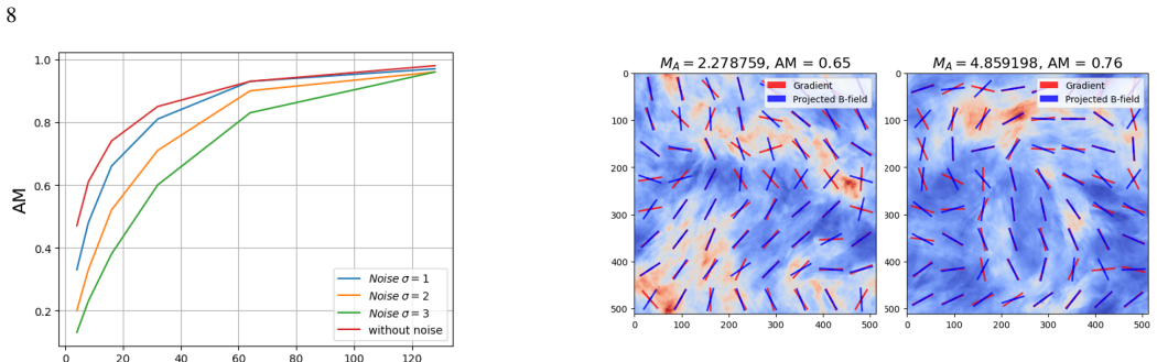
- [Section 6; Figures 2-3; Table 1] The central claim that SIGs trace the magnetic field well 'both when the observations resolve and do not resolve the Alfvén scale lA' is not established by the presented data. The main AM results in Figure 3 use a fixed block size of 64² for every simulation, while Table 1 gives lA/Δx = 37.0 (M1), 21.0 (M2), 15.6 (M3), 3.64 (M4), and 1.07 (M5). Because 64 pixels is larger than lA in all five cases, the Figure 3 bottom panel tests only the unresolved branch. Figure 2, the only scan with blocks smaller than lA (4², 8², 16², 32² for M1), reports only that AM rises from 0.4 at 4² to 0.93 at 64²; the intermediate values, including 32² (which is still below lA = 37Δx), are not given, and the text notes that 4² is below the numerical dissipation scale. Consequently, the paper does not show AM ≈ 0.9 when observations resolve lA, and the Section 6 statement that 'we do not have rigid constraints on the required resolution of observations' overstates the implications. Please report AM as a function of block size normalized by lA for all simulations, or explicitly restrict the claim to the unresolved regime.
- [Section 5.3; Eq. (10); Figure 8] The X-ray gradient result is not quantitatively supported. The text says that GT can be successfully applied to X-ray maps and that the AM is 'significant enough', but no AM values, error bars, or noise levels are reported for Figure 8. In addition, the section does not state the sub-block size used for the X-ray maps; assuming the same fixed 64² block as in Section 4.2, the A1 and A2 runs have lA = 42.1Δx and 4.62Δx (Table 2), so the X-ray test would also cover only the unresolved regime. To support the Section 6 claim that the removal of the resolving-lA constraint applies to X-ray tracing, the authors should provide quantified AM values for resolved block sizes or explicitly limit the claim to the unresolved regime.
- [Section 4.1; Eq. (8); Section 5] The synthetic-observation validation relies on two simplifying emission-model assumptions that are not stress-tested: the cosmic-ray density is taken to be constant along the line of sight, and the synchrotron emissivity index is fixed at γ = 2 in Eq. (8). The X-ray maps furthermore assume I ∝ n² (Eq. 10). Real intracluster media may have cosmic-ray density fluctuations, nonthermal components, or emission processes not captured by these scalings, any of which could alter the relation between intensity gradients and the magnetic field. Because the stated goal is to justify ICM applications, the paper should either test the sensitivity (for example by adding CR fluctuations or varying γ) or explicitly list these emissions assumptions as limitations of the present simulation evidence.
- [Section 4.2; Figure 3] The reported AM ≈ 0.9 for each simulation appears to be a single value with no uncertainty estimate. Without error bars computed across sub-blocks or over multiple snapshots, the claimed 'only weakly depends on MA' cannot be distinguished from snapshot-to-snapshot or map-to-map noise. Please add uncertainties, or at least state how many independent sub-blocks were used to compute each AM value.
minor comments (6)
- [Throughout] The manuscript contains numerous typos; for example, Table 3 lists 'Aligment Measrure' and 'Techinque', and Section 2.1 reads 'dominated by the dominated by Alfvénic modes'.
- [Equation (8), Section 4.1] The electron distribution is written as 'N(E)E ∼ E^α dE', which is likely a typo for N(E)dE ∝ E^α dE; in addition, the sentence about 'α = 3, which gives γ' is confusing and should be clarified.
- [Figure 4 caption] The vertical axis is described as 'the relative degree between individual gradient vector directions'; this should be the angle between the individual gradient vectors and the projected magnetic field.
- [Figure 8 caption] The caption refers to 'polarization vector' for X-ray maps, but X-ray emission is unpolarized in this model; the vectors shown are presumably the projected magnetic field direction, and the caption should say so.
- [Section 5.1, Figure 6] The noise test is presented visually only; adding the AM values for the three noise levels and for the different block sizes would make the claimed degradation quantitative.
- [Section 4.2] The sentence 'We construct a synthetic observation for synchrotron intensity (the method described at sec. 3)' should refer to Section 4.1 rather than Section 3, since the construction of the synchrotron map is introduced in Section 4.1.
Circularity Check
No circular reduction is exhibited: the paper is a numerical validation whose synthetic maps are built from the same simulation fields it recovers; the main defect is a resolution-support gap in the 'resolve lA' claim, which is a scope problem, not circularity.
full rationale
This paper is not an analytic derivation; its central claim is an empirical alignment measurement on synthetic observations. The signal maps (Eq. 8, I_sync proportional to the line-of-sight integral of B_POS^gamma, and Eq. 10, I_X proportional to the integral of n^2) and the ground-truth projected magnetic field come from the same simulation, so the test is an internal consistency check rather than an external benchmark. That limits how much the result can validate the technique against reality, but it is not a circular reduction: no parameter is fitted so as to force AM about 0.9, and the gradients could in principle fail to align with the projected field even though both are functionals of the same B field. The scaling lA = L M_A^{-3} (Eq. 6, cited to Lazarian 2006) is an input physical assumption of the analysis, not a conclusion derived from the target alignment result, and the sub-block averaging procedure is adopted as methodology from prior gradient-technique papers rather than as an imported uniqueness theorem. There is, however, a significant support gap that should be flagged in the verdict: Section 6 states that 'SIGs trace the magnetic field well both when the observations resolve and do not resolve the Alfvén scale lA,' but all main AM numbers (Figure 3, bottom panel) are obtained with a fixed 64^2 block. With lA/Delta x equal to 37.0, 21.0, 15.6, 3.64, and 1.07 for M1 through M5 (Table 1), a 64 Delta x block is larger than lA in every simulation, so the main reported AM values cover only the regime where the observational block does not resolve lA. The resolved branch appears only in the Figure 2 block-size scan for M1, where the AM values for the resolved block sizes are not quoted in the text and the 4^2 block is explicitly said to be below the numerical dissipation scale. The X-ray runs have the same issue: A1 has lA/Delta x = 42.1 and A2 has 4.62, but the same 64^2 block leaves both cases unresolved. This weakens the breadth of the paper's central resolution claim, but it does not make the reported alignment a tautology or a fit in disguise. Because the central validation is self-contained but internal, and the few self-citations are not load-bearing reductions, the circularity score is low.
Assumptions & free parameters
free parameters (3)
- Sub-block averaging size =
64 by 64 pixels
- Synchrotron emissivity index gamma =
2
- Noise injection levels =
1, 2, and 3 sigma of map intensity
assumptions (6)
- domain assumption Critical balance and scale-dependent anisotropy (GS95, LV99): turbulent eddies are elongated along the local magnetic field, so gradients of velocity and magnetic field are perpendicular to the field.
- domain assumption Weakly compressible approximation: the intracluster medium is subsonic, so incompressible simulations with Ms=0 capture the relevant behavior.
- domain assumption Synchrotron intensity depends only on the magnetic field, with negligible cosmic-ray density fluctuations on the scales of field variations.
- domain assumption Density fluctuations mimic velocity fluctuations in subsonic turbulence, so density (X-ray) gradients can proxy velocity gradients.
- domain assumption X-ray emissivity is proportional to n^2, the thermal emission measure.
- domain assumption Nonlinear turbulent dynamo transfers only a small fraction (3/38) of the energy cascade into magnetic energy and can be neglected in the super-Alfvenic regime.
Cite this review
Pith. "Pith review of Tracing magnetic field in super-Alfvenic turbulence with Gradient Technique." pith.science (2026). https://pith.science/paper/G3UOZC6X
@misc{pith2026241202102,
  author       = {Pith},
  title        = {Pith review of: Tracing magnetic field in super-Alfvenic turbulence with Gradient Technique},
  year         = {2026},
  howpublished = {\url{https://pith.science/paper/G3UOZC6X}},
  note         = {Machine review of arXiv:2412.02102}
}
read the original abstract
Super-Alfvenic turbulence is important for many astrophysical objects, particularly galaxy clusters. In this paper, we explore the accuracy of Synchrotron Intensity Gradients (SIGs) and X-ray intensity gradients to map magnetic fields in super-Alfvenic turbulence for a set of astrophysically relevant parameters of turbulent driving. Analyzing our synthetic observations, we report a good accuracy for both techniques. Our results are suggestive that other types of Gradient Technique (GT) can be successfully employed to trace magnetic fields within super-Alfvenic sub-sonic turbulence.
Figures


Figures from the paper (3 more)


Reference graph
Works this paper leans on
-
[1]
, " * write output.state after.block = add.period write newline
ENTRY address archivePrefix author booktitle chapter doi edition editor eprint howpublished institution journal key month number organization pages publisher school series title misctitle type volume year version url label extra.label sort.label short.list INTEGERS output.state before.all mid.sentence after.sentence after.block FUNCTION init.state.consts ...
-
[2]
write newline
" write newline "" before.all 'output.state := FUNCTION format.url url empty "" new.block "" url * "" * if FUNCTION format.eprint eprint empty "" archivePrefix empty "" archivePrefix "arXiv" = new.block " " eprint * " " * new.block " " eprint * " " * if if if FUNCTION format.doi doi empty "" " " doi * " " * if FUNCTION format.pid doi empty eprint empty ur...
-
[3]
9tEXtSoftwareMatplotlib version3.3.4, https://matplotlib.org/ T̺ pHYs a a ?iLIDATxyxSe ;IӤ -Բ 8#V QA :˰T pG q ZYd( ʾt4m& 4R64 KrrN䡴 B
thebibliography [1] 20pt to REFERENCES 6pt =0pt 10pt plus 3pt =0pt =0pt =1pt plus 1pt =0pt =0pt -12pt =13pt plus 1pt =20pt =13pt plus 1pt \@M =10000 =-1.0em =0pt =0pt 0pt =0pt =1.0em @enumiv\@empty 10000 10000 `\.\@m \@noitemerr \@latex@warning Empty `thebibliography' environment \@ifnextchar \@reference \@latexerr Missing key on reference command Each re...
2019
-
[4]
1999, Physics of Fluids, 11, 1880, 10.1063/1.870050
Alvelius , K. 1999, Physics of Fluids, 11, 1880, 10.1063/1.870050
doi:10.1063/1.870050 1999
-
[5]
G., Lazarian , A., & Vaillancourt , J
Andersson , B. G., Lazarian , A., & Vaillancourt , J. E. 2015, , 53, 501, 10.1146/annurev-astro-082214-122414
-
[6]
1996, , 34, 155, 10.1146/annurev.astro.34.1.155
Beck , R., Brandenburg , A., Moss , D., Shukurov , A., & Sokoloff , D. 1996, , 34, 155, 10.1146/annurev.astro.34.1.155
-
[7]
2019, Turbulence in Magnetohydrodynamics
Beresnyak , A., & Lazarian , A. 2019, Turbulence in Magnetohydrodynamics
work page 2019
-
[8]
Bezanson, J., Edelman, A., Karpinski, S., & Shah, V. B. 2017, SIAM review, 59, 65. https://doi.org/10.1137/141000671
Show all 65 references
-
[9]
2010, , 513, A30, 10.1051/0004-6361/200913696
Bonafede , A., Feretti , L., Murgia , M., et al. 2010, , 513, A30, 10.1051/0004-6361/200913696
2010 doi
-
[10]
H., & Kennedy, C
Carpenter, M. H., & Kennedy, C. A. 1994, Fourth-order 2N-storage Runge–Kutta schemes, Technical Report NASA TM-109112, NASA Langley Research Center, VA
1994
-
[11]
2002, , 88, 245001, 10.1103/PhysRevLett.88.245001
Cho , J., & Lazarian , A. 2002, , 88, 245001, 10.1103/PhysRevLett.88.245001
2002 doi
-
[12]
2003, , 345, 325, 10.1046/j.1365-8711.2003.06941.x
---. 2003, , 345, 325, 10.1046/j.1365-8711.2003.06941.x
2003
-
[13]
Cho , J., & Vishniac , E. T. 2000, , 539, 273, 10.1086/309213
2000 doi
-
[14]
C., Wagner, G
Constantinou, N. C., Wagner, G. L., Palóczy, A., et al. 2023, FourierFlows/FourierFlows.jl: v0.10.3, v0.10.3, Zenodo, 10.5281/zenodo.7631539
2023 doi
-
[15]
M., Hakobian , N., & Troland , T
Crutcher , R. M., Hakobian , N., & Troland , T. H. 2010, , 402, L64, 10.1111/j.1745-3933.2009.00802.x
2010
-
[16]
Davidson, P. A. 2015, Turbulence: An Introduction for Scientists and Engineers, 2nd edn. (Oxford University Press)
2015
-
[17]
Draine , B. T. 2006, , 636, 1114, 10.1086/498130
2006 doi
-
[18]
P., Falcke , H., Karuppusamy , R., et al
Eatough , R. P., Falcke , H., Karuppusamy , R., et al. 2013, , 501, 391, 10.1038/nature12499
2013 doi
- [19]
-
[20]
Fletcher, M. T. 2015, Master's thesis, Naval Postgraduate School, Monterey, CA
2015
-
[21]
M., Haverkorn , M., Staveley-Smith , L., et al
Gaensler , B. M., Haverkorn , M., Staveley-Smith , L., et al. 2005, Science, 307, 1610, 10.1126/science.1108832
2005 doi
-
[22]
V., Newell , A
Galtier , S., Nazarenko , S. V., Newell , A. C., & Pouquet , A. 2000, Journal of Plasma Physics, 63, 447, 10.1017/S0022377899008284
2000 doi
-
[23]
Goldreich , P., & Kylafis , N. D. 1981, , 243, L75, 10.1086/183446
1981 doi
-
[24]
1995, , 438, 763, 10.1086/175121
Goldreich , P., & Sridhar , S. 1995, , 438, 763, 10.1086/175121
1995 doi
-
[25]
F., & Lazarian , A
Gonz \'a lez-Casanova , D. F., & Lazarian , A. 2017, , 835, 41, 10.3847/1538-4357/835/1/41
2017 doi
-
[26]
Ho, K. W. 2022, MHDFlows.jl, 0.2.1b, Zenodo, 10.5281/zenodo.8242702
2022 doi
- [27]
-
[28]
W., Yuen , K
Ho , K. W., Yuen , K. H., Leung , P. K., & Lazarian , A. 2019, , 887, 258, 10.3847/1538-4357/ab578c
2019 doi
- [29]
- [30]
-
[31]
2022, , 941, 92, 10.3847/1538-4357/ac9df0
Hu , Y., Lazarian , A., Beck , R., & Xu , S. 2022, , 941, 92, 10.3847/1538-4357/ac9df0
2022 doi
-
[33]
2020 b , , 901, 162, 10.3847/1538-4357/abb1c3
---. 2020 b , , 901, 162, 10.3847/1538-4357/abb1c3
2020 doi
-
[34]
2024, Nature Communications, 15, 1006, 10.1038/s41467-024-45164-8
Hu , Y., Stuardi , C., Lazarian , A., et al. 2024, Nature Communications, 15, 1006, 10.1038/s41467-024-45164-8
2024 doi
-
[35]
2021, , 911, 37, 10.3847/1538-4357/abea18
Hu , Y., Xu , S., & Lazarian , A. 2021, , 911, 37, 10.3847/1538-4357/abea18
2021 doi
-
[36]
H., & Lazarian , A
Hu , Y., Yuen , K. H., & Lazarian , A. 2019, , 886, 17, 10.3847/1538-4357/ab4b5e
2019 doi
-
[37]
Hunter , J. D. 2007, Computing in Science and Engineering, 9, 90, 10.1109/MCSE.2007.55
2007 doi
-
[38]
Jokipii , J. R. 1966, , 146, 480, 10.1086/148912
1966 doi
-
[39]
D., Rudnick , L., et al
Knowles , K., Cotton , W. D., Rudnick , L., et al. 2022, , 657, A56, 10.1051/0004-6361/202141488
2022 doi
-
[40]
Kraichnan , R. H. 1965, Physics of Fluids, 8, 1385, 10.1063/1.1761412
1965 doi
-
[41]
2006, Astronomische Nachrichten, 327, 609, 10.1002/asna.200610603
Lazarian , A. 2006, Astronomische Nachrichten, 327, 609, 10.1002/asna.200610603
2006 doi
-
[42]
2007, Journal of Quantitative Spectroscopy and Radiative Transfer, 106, 225, 10.1016/j.jqsrt.2007.01.038
---. 2007, Journal of Quantitative Spectroscopy and Radiative Transfer, 106, 225, 10.1016/j.jqsrt.2007.01.038
2007 doi
-
[43]
2007, , 378, 910, 10.1111/j.1365-2966.2007.11817.x
Lazarian , A., & Hoang , T. 2007, , 378, 910, 10.1111/j.1365-2966.2007.11817.x
2007
- [44]
-
[45]
2012, , 747, 5, 10.1088/0004-637X/747/1/5
Lazarian , A., & Pogosyan , D. 2012, , 747, 5, 10.1088/0004-637X/747/1/5
2012 doi
-
[46]
2016, , 818, 178, 10.3847/0004-637X/818/2/178
---. 2016, , 818, 178, 10.3847/0004-637X/818/2/178
2016 doi
-
[47]
Lazarian , A., & Vishniac , E. T. 1999, , 517, 700, 10.1086/307233
1999 doi
-
[48]
Lazarian , A., & Yuen , K. H. 2018 a , , 865, 59, 10.3847/1538-4357/aad3ca
2018 doi
-
[49]
2018 b , , 853, 96, 10.3847/1538-4357/aaa241
---. 2018 b , , 853, 96, 10.3847/1538-4357/aaa241
2018 doi
-
[50]
H., Lee , H., & Cho , J
Lazarian , A., Yuen , K. H., Lee , H., & Cho , J. 2017, , 842, 30, 10.3847/1538-4357/aa74c6
2017 doi
-
[51]
2001, , 562, 279, 10.1086/323470
Lithwick , Y., & Goldreich , P. 2001, , 562, 279, 10.1086/323470
2001 doi
-
[52]
Mac Low , M.-M., & Klessen , R. S. 2004, Reviews of Modern Physics, 76, 125, 10.1103/RevModPhys.76.125
2004 doi
-
[53]
2001, , 554, 1175, 10.1086/321413
Maron , J., & Goldreich , P. 2001, , 554, 1175, 10.1086/321413
2001 doi
-
[54]
F., & Ostriker , E
McKee , C. F., & Ostriker , E. C. 2007, , 45, 565, 10.1146/annurev.astro.45.051806.110602
2007 arXiv
-
[55]
2020, , 498, 3125, 10.1093/mnras/staa2530
Pakmor , R., van de Voort , F., Bieri , R., et al. 2020, , 498, 3125, 10.1093/mnras/staa2530
2020 doi
-
[56]
M., Tomida , K., White , C
Stone , J. M., Tomida , K., White , C. J., & Felker , K. G. 2020, , 249, 4, 10.3847/1538-4365/ab929b
2020 doi
-
[57]
N., & Hoang , T
Tram , L. N., & Hoang , T. 2022, Frontiers in Astronomy and Space Sciences, 9, 923927, 10.3389/fspas.2022.923927
2022
-
[58]
Vogt , C., & En lin , T. A. 2003, , 412, 373, 10.1051/0004-6361:20031434
2003 doi
-
[59]
2016, , 833, 215, 10.3847/1538-4357/833/2/215
Xu , S., & Lazarian , A. 2016, , 833, 215, 10.3847/1538-4357/833/2/215
2016 doi
-
[60]
2002, Physical Review Letters, 89, B1102+, 10.1103/PhysRevLett.89.281102
Yan , H., & Lazarian , A. 2002, Physical Review Letters, 89, B1102+, 10.1103/PhysRevLett.89.281102
2002 doi
- [61]
- [62]
-
[63]
2010, Highlights of Astronomy, 15, 446, 10.1017/S1743921310010215
---. 2010, Highlights of Astronomy, 15, 446, 10.1017/S1743921310010215
2010 doi
-
[64]
H., & Lazarian , A
Yuen , K. H., & Lazarian , A. 2017, , 837, L24, 10.3847/2041-8213/aa6255
2017 doi
-
[65]
2020, , 895, 20, 10.3847/1538-4357/ab88ac
Zhang , J.-F., Hu , K., Cho , J., & Lazarian , A. 2020, , 895, 20, 10.3847/1538-4357/ab88ac
2020 doi
-
[66]
W., et al
Zhang , J.-F., Lazarian , A., Ho , K. W., et al. 2019, , 486, 4813, 10.1093/mnras/stz1176
2019 doi
Reviewed August 11, 2026 · model on record in the stance chip above.
Discussion (0). Continue with ORCID to comment.