Dynamical Persistent Homology via Wasserstein Gradient Flow

Jinhui Xu; Minghua Wang

REVIEW 5 major objections 7 minor 41 references

Dynamical Persistent Homology via Wasserstein Gradient Flow

T0 review · 5 major / 7 minor · reviewed 2026-08-11 · deepseek-v4-flash

Challenge this review Re-run · record.json Download PDF Read on arXiv ↗ Review JSON

Pith's one-line read This paper claims that persistence diagrams can be driven along Wasserstein geodesics by editing the underlying data through a gradient update of the filtration.

desk verdict Pleasantly motivated but not ready: the geodesic guarantee is unproved, Algorithm 2's pseudocode returns a constant sequence, and the experiments are qualitative. read the letter →

arxiv 2412.03806 v1 pith:BYVWJIHL submitted 2024-12-05 math.AT cs.CG

Minghua Wang , Jinhui Xu This is my paper · ORCID

classification math.ATcs.CG MSC 55N3149Q22

keywords persistenthomologypersistencediagramWassersteingradientflowoptimaltransportMcCanninterpolationJKOschemetopologicaldataanalysisfiltrationoptimization

verification ladder T0 review T1 audit T2 compute T3 formal

The pith

A machine-rendered reading of the paper's core claim, the machinery that carries it, and where it could break.

The reading

The paper tries to establish that variations in persistence diagrams can be translated back into changes of the underlying data, by treating the diagram as a probability measure and letting it evolve along a Wasserstein gradient flow. If true, this replaces the one-way data-to-diagram pipeline with a loop in which a user prescribes a target diagram (or an energy) and the data is edited so its topological summary follows a geodesic in Wasserstein space. The two proposed algorithms—one based on McCann interpolation toward a fixed target, one based on the JKO scheme with an energy functional—each couple the diagram's motion to the filtration by a differentiable critical-set update. The paper demonstrates the idea on circle denoising and circle emergence, and identifies scalability, statistical theory, and loss conflicts as open limitations.

What carries the argument

The central objects are McCann interpolation—the displacement interpolation between two probability measures along the optimal transport map, which yields a geodesic in Wasserstein space—and the Jordan–Kinderlehrer–Otto (JKO) scheme, a time-discretized Wasserstein gradient flow. Persistence diagrams are represented as equally weighted empirical measures in the Euclidean plane, and the critical-set gradient method supplies the update that turns an abstract diagram movement into a concrete change of the filtration function on the simplicial complex.

What would settle it

Count the number of off-diagonal birth–death pairs in the 1st persistence diagram while Algorithm 2 runs on uniformly random points; because the JKO target is initialized with the same number of atoms as the current diagram, the count cannot increase, so a genuinely new circle pair emerging from the diagonal would contradict the algorithm's stated mechanism.

Watch

Extended reading notes

Core claim

The central claim is that the one-way pipeline from data to persistence diagram can be reversed by viewing a persistence diagram as an empirical probability measure with equal weights at the birth–death points and running a Wasserstein gradient flow on it. Given a target diagram, the first algorithm uses the optimal transport plan between the current diagram and the target to form a McCann displacement interpolation, then adjusts the filtration function with a critical-set gradient method so the data's computed diagram tracks the interpolated diagram. Without a target, the second algorithm applies one JKO step of an energy functional to the current diagram, then performs the same filtration update. The paper demonstrates both schemes on a noisy circle (denoising) and on random points (circle emergence), claiming the diagrams evolve along $W_2$ geodesics whenever the targets are achievable at each step.

Load-bearing premise

The framework assumes persistence diagrams are just finite equally weighted point sets in the plane, that the standard $W_2$ metric governs their motion, and that the desired target diagram can actually be reached at each optimization step.

Editorial extensions

If this is right

With a known target diagram, the McCann-based algorithm makes the persistence diagram evolve along a Wasserstein geodesic toward the target whenever the target is reachable at every step.
Without a target diagram, the JKO-based algorithm lets an energy functional steer the persistence diagram, initializing the target at the current diagram so the number of persistence pairs is fixed.
The filtration update via the critical-set method means each optimization step edits the original data (point cloud, graph, or image) rather than the diagram directly.
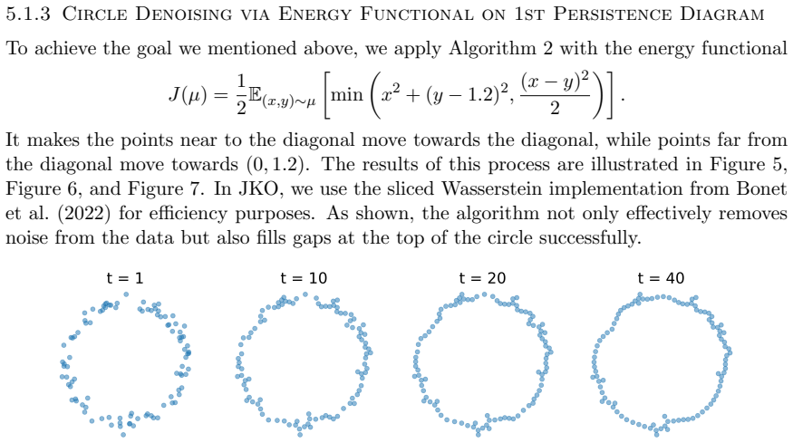
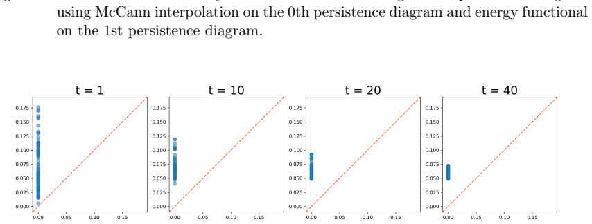
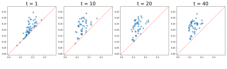
In the circle-denoising case, combining the two algorithms removes noise from the 0th persistence diagram and fills a gap in the 1st persistence diagram, making the underlying circle explicit.
In the circle-emerging case, uniformly random points are rearranged so a first-homology circle appears, showing the method can amplify a weak topological signal.

Reading between the lines

Editorial extensions of the paper, not claims the author makes directly.

An extension the paper leaves implicit: because the JKO algorithm fixes the number of persistence pairs, any apparent creation or destruction of off-diagonal pairs must actually come from the energy functional moving near-diagonal pairs across the diagonal; a direct test would be to count off-diagonal pairs over time.
The same flow formulation could be applied to other persistence summaries, such as zigzag or multiparameter persistence, if a suitable metric and a differentiable projection back to data are available.
Replacing the exact optimal transport plan with an entropy-regularized Sinkhorn plan would give a smoothed McCann interpolation, potentially improving numerical stability for large diagrams.
The guarantee degrades gracefully if the target diagram is not achievable at every step; measuring the gap between the interpolated diagram and the diagram actually realized by the updated filtration would quantify how much of the geodesic property survives.

Share X Bluesky LinkedIn Reddit HN

Editorial analysis

A structured set of objections, weighed in public.

Desk editor's note, referee report, and a circularity audit.

Desk Editor's Note

read the letter

Quick take: the idea is plausible but the paper does not support it. What is actually new is coupling OT-derived intermediate persistence diagrams (McCann interpolation or JKO steps) with the Nigmetov-Morozov big-step critical-set optimizer to back-propagate diagram changes into filtration values. That is a real extension of Gameiro et al. and Carriere et al., and the two toy experiments show the intended behavior. I also give credit for a limitations section that names missing statistical theory, GPU scalability, and unresolved singleton-loss conflicts.

The soft spots are load-bearing. Algorithm 1 claims the measure µt moves along the W2 geodesic to the target diagram. But the update uses the barycentric projection of the Sinkhorn plan, Eq. 13, not the McCann interpolation. McCann needs an optimal transport map between two measures of equal mass; when n≠m or the Sinkhorn plan splits mass, X1 is not the target and uniform(X1) is not Z. So the algorithm is interpolating toward a projection of the target, not the target, and the claimed geodesic property is unproved and generally false. The caveat "provided the target is achievable" does not fix this.

Algorithm 2 has a more basic problem. The number of atoms is fixed at n for all k, so the measure update cannot create or destroy off-diagonal persistence pairs. The circle-emerging experiment depends on changing which H1 features survive, so the mechanism cannot be doing what the figure suggests. Worse, the pseudocode initializes y_i from x_i and never updates y_i after the JKO step; line 8 sets Y(k) to the stale y_i, so Algorithm 2 as written returns Y(k)=X(k). That is an internal contradiction, not a minor typo, because the JKO solution on line 7 is discarded.

The experiments are qualitative: two 2D examples, no baselines, no error bars, no code or data. For a methods paper that's thin even when the theory is solid. Here the theory is not solid.

Overall: I see a worthwhile heuristic and a lot of work needed. The framing of persistence diagrams as equally weighted empirical measures in R^2 is a mismatch for the persistence-diagram metric with its diagonal, and the paper never confronts that. The idea might be salvageable by restricting to equal-cardinality matched diagrams or by explicitly treating the diagonal, and then proving when the critical-set optimizer can realize the interpolation. As it stands, I would not send this to peer review; I'd desk reject and suggest the authors resubmit after fixing the algorithms and adding quantitative evidence.

Referee Report

5 major / 7 minor

Summary. The manuscript proposes two methods for adapting a filtration function on a simplicial complex so that the resulting persistence diagrams evolve in a prescribed way. Algorithm 1 uses Sinkhorn barycenters to define an interpolation between the current persistence diagram and a user-specified target diagram, and then fits the filtration to the interpolated diagram using the critical-set method of Nigmetov and Morozov. Algorithm 2 replaces the target diagram by one obtained from a JKO step of a manually chosen energy functional. Two case studies (circle denoising and circle emerging) are presented, with figures showing point clouds and persistence diagrams over iterations.

Significance. If the central claim were correct, the paper would offer a principled way to invert the map from data to persistence diagrams, enabling direct manipulation of data guided by Wasserstein dynamics in diagram space. The paper builds on recent differentiable-persistence tools (Nigmetov and Morozov; Carriere et al.) and provides illustrative computational experiments. However, as detailed below, the main theoretical guarantee is not proven and is in fact false for the algorithm as written, and the second algorithm's pseudocode does not implement the claimed JKO dynamics. The paper also lacks any quantitative evaluation. The strengths are the clear presentation of background material and the use of state-of-the-art computational components (Sinkhorn, sliced Wasserstein, big-step topological optimization), but these do not compensate for the load-bearing rigor gaps.

major comments (5)

[Section 4.1, Eq. (13), Algorithm 1 lines 5-7] The claimed guarantee that μ_t evolves along the W2-geodesic to Z is not established and is generally false. The update X1_i = (Σ_j π_ij z_j)/(Σ_j π_ij) is the barycentric projection of the target through the Sinkhorn plan, not the image of Z under the optimal transport map. McCann's theorem applies to the interpolation between μ_k and the push-forward of μ_k under the optimal map; it does not apply to a barycentric projection unless π is a permutation matrix with n=m and no split mass. In the typical case n≠m, X1 is not a measure equal to Z and the interpolation is between μ_k and uniform(X1), not toward Z. Moreover, even when Z is achievable, Equation (13) projects each source point to a weighted average of target points; the resulting empirical measure is not Z, so the sequence X(k) does not converge to Z in general. The phrase 'provided that the target persistence diagram is achievable at each step' is also circular because the paper gives no characterization of achievability and the authors explicitly state (Section 4.1) that the learnable scheme cannot guarantee that the persistence diagram is always achievable. Thus the geodesic guarantee is not proven and cannot be checked.
[Section 4.2, Algorithm 2 lines 4-8] The pseudocode does not propagate the JKO solution to Y(k). Line 4 initializes (y_1,...,y_n) to (x_1,...,x_n); line 7 computes a new measure μ as the argmin; but line 8 then sets Y(k) = {y_i^(k)}, the unchanged initial values. As written, Y(k) = X(k) at every iteration, so the inner filtration-fitting loop fits the current diagram to itself and no dynamics occur. If the intended assignment was to take the support of the argmin measure, this must be stated explicitly, together with a proof that this support forms a valid persistence diagram and that the resulting cardinality can change. Without such a correction, Algorithm 2 is not a meaningful implementation of the JKO scheme.
[Section 4.2 and Section 5.2] The fixed-cardinality formulation is incompatible with the circle-emerging experiment. Algorithm 2 initializes the target measure with the same n points as the current diagram and, if restricted to n-point measures, the JKO step can only move existing points; it cannot create new off-diagonal persistence pairs. Yet the circle-emerging experiment (Section 5.2) aims to create H1 features that are absent from the initial random point cloud. The paper never explains how the extra H1 pairs appear, so the reported results cannot be attributed to the algorithm as described. This is a fundamental mismatch between the algorithm's representational constraints and the experimental goal.
[Sections 3.3 and 4.1] The paper models a persistence diagram as an empirical measure with total mass 1 on the off-diagonal points. This is not the standard Wasserstein geometry of persistence diagrams, where the diagonal is a separate set with its own multiplicity and mass can be transported to and from the diagonal. Consequently, the 'Wasserstein gradient flow' discussed is a flow in P2(R^2), not a flow in the space of persistence diagrams under the usual W2 metric. The authors neither justify this choice nor relate it to stability properties of persistence diagrams, so the topological relevance of the construction is left unjustified.
[Section 5] There are no quantitative results. The case studies are qualitative figure sequences; no convergence curves, error bars, runtime measurements, or comparisons with prior methods are provided. The hyperparameters t_k, η, τ, ϵ, and the energy functionals are not listed, and no sensitivity analysis is given. Thus the empirical claims cannot be verified or reproduced from the manuscript.

minor comments (7)

[Section 1] There is a typo: 'analyais' should be 'analysis'.
[Section 2] The sentence 'Recent work has shifted focus to the use of p-Wasserstein distances, A central challenge...' has a capitalization and run-on issue; it should be split into two sentences.
[Section 3.4] The JKO formula displays 'W 2 2 (µ, µk)' with inconsistent sub/superscript formatting; it should be written as W_2^2(µ, µk) throughout.
[Section 5.1.1] The repulsion loss formula is ambiguous: the expression '1/∥σi − σj∥2 + ϵ' lacks parentheses; the intended formula is likely Σ_i Σ_{j≠i} 1/(∥σi − σj∥^2 + ϵ).
[Algorithms 1 and 2] The symbol f is used both for the filtration function and for the update 'f ← f − η∇f'; the update is not clearly defined for the simplicial complex K, since the critical-set method of Nigmetov and Morozov returns a filtration function, but the manuscript does not specify how the update is applied to all simplices.
[Section 5.2] The target for the 1st persistence diagram in the circle-emerging experiment is not specified explicitly; the text says 'enhance the circles' but gives no birth-death coordinates, unlike the 0th diagram target (0, 0.08). A precise target would improve reproducibility.
[References] The reference 'Wang et al.' in the Related Work section is incomplete: it lacks a year, venue, and full author list.

Circularity Check

2 steps flagged · score 6.0 of 10

Algorithm 1's geodesic guarantee is the algorithm's own target construction rather than a derived result, and Algorithm 2 similarly imposes hand-picked energy flows by fitting to generated targets.

self definitional [Section 4.1, Algorithm 1 (lines 6–10 and paragraph after the algorithm)]
"X1 ← TargetDgm(π) ▷ Use Equation (13); Y (k) ← (1 − t)X (k) + tX1 ▷ Use McCann Interpolation ... L ←Loss(dgmp(K, f), Y(k)); ∇f ← CriticalSetMethod(L, f); f ← f − η∇f ... our algorithm guarantees that the measure µt evolves along the geodesic in Wasserstein space, provided that the target persistence diagram is achievable at each step."

The geodesic guarantee is essentially the definition of Y(k): the target is constructed as an interpolation, and the loss is minimized so that dgmp matches Y(k). Conditional on exact achievability, the persistence diagram evolution equals the constructed Y(k) sequence by construction, so the claim is a restatement of the algorithm's own objective rather than a derived dynamical property. The load-bearing identification of Eq. (13) with McCann interpolation is what would make the theorem applicable, but Eq. (13) is a barycentric projection through the Sinkhorn plan, not the image of the target under an optimal transport map, so the geodesic statement is an asserted property of the constructed target, not a consequence of Theorem 2.
fitted input called prediction [Section 4.2, Algorithm 2 (lines 4–8) and the case illustrations in Sections 5.1.3 and 5.2]
"(y(k)_1, y(k)_2, . . . , y(k)_n) ← (x(k)_1, x(k)_2, . . . , x(k)_n); µk ← (1/n) Σ δ_x(k)_i; µ ← argmin_µ (1/(2τ)) W_2^2(µk, µ) + J(µ); Y (k) ← {y(k)_i}_{i=1}^n ... we initialize the target persistence diagram with the current persistence diagram, ensuring equal cardinalities."

The target persistence diagram at each step is generated by a JKO step of the user-chosen energy functional J, and then the filtration is fitted to that target through the same critical-set loss. The resulting 'dynamical persistence diagram' is therefore the hand-picked energy's flow imposed through the fitting objective; the circle denoising and circle emerging evolutions in Section 5 demonstrate the chosen J rather than an independent prediction from the data. The fixed cardinality n, inherited from the initialization, also prevents creation or destruction of off-diagonal persistence pairs, so the reported evolution is additionally constrained by the algorithm's own cardinality assumption.

full rationale

The paper contains no load-bearing self-citation chain, and the main algorithmic workhorse (the critical-set filtration update) is taken from the external, independently developed method of Nigmetov and Morozov. The related-work citations to the authors' own papers are not used to justify the central construction. However, the paper's central theoretical claim that the measure follows the Wasserstein geodesic is not derived from an external law: Algorithm 1 defines Y(k) as an interpolation toward a target and then fits the filtration to Y(k), so the geodesic motion is true only in the tautological sense that the algorithm's own target sequence is the interpolation, and only if the fitting succeeds. Algorithm 2 likewise generates its target by a JKO step of a hand-selected energy and then fits to it, so the reported dynamics are the imposed objective, not discovered from data. A separate correctness concern, noted in the steps, is that Eq. (13) is a barycentric projection through a Sinkhorn plan rather than a McCann displacement interpolation when n ≠ m or when mass splits, so the claimed geodesic property does not actually follow from the cited theorem. For circularity purposes, the key issue is that the geodesic and Wasserstein-gradient-flow evolutions are constructed into the algorithm's objective, making the central claims at least partially circular by construction. The score is therefore 6 rather than higher because the paper is otherwise self-contained and does not rely on a self-citation chain or a uniqueness import.

Assumptions & free parameters 7 free parameters · 6 assumptions · 1 invented entities

The central algorithms rest on three kinds of unpaid inputs: hand-chosen targets and schedules (interpolation step t_k, learning rate, JKO step, energy functionals, H0 targets), assumptions that persistence diagrams behave like equally weighted Euclidean measures under W2, and assumptions that the critical set method can realize any target diagram and that Eq. (13) is a McCann interpolation. Algorithm 2 additionally assumes fixed cardinality is sufficient for topological dynamics, which conflicts with the need to create or destroy off-diagonal features.

free parameters (7)

McCann interpolation step size t_k = t = 1/(K-k+1)
Hand-chosen decreasing schedule in Algorithm 1; no justification or sensitivity analysis.
filtration learning rate eta = unspecified
Used in lines 12-13 of Algorithms 1 and 2 but not listed in inputs or assigned a value.
JKO time step tau = unspecified
Input to Algorithm 2 with no recommended value or tuning rule.
energy functional J for circle denoising = J(mu) = (1/2) E[min(x^2+(y-1.2)^2, (x-y)^2/2)]
Hand-designed in Section 5.1.3 to move points toward the diagonal or (0,1.2); the choices encode the desired outcome.
energy functional J for circle emerging = J(mu) = (1/4) E[(y-(x+0.15))^2 + x^2]
Hand-designed in Section 5.2 to push first persistence pairs away from the diagonal and left; no selection principle.
target H0 birth-death coordinates = (0,0.05) in Section 5.1.2; (0,0.08) in Section 5.2
User-specified target persistence values used as Z in Algorithm 1; results depend on these.
repulsion loss epsilon = small positive constant
Introduced in Section 5.1.1 to prevent division by zero; exact value omitted.

assumptions (6)

standard math Benamou-Brenier theorem and McCann interpolation theorem
Background optimal transport results invoked in Section 4.1.
domain assumption Persistence diagrams are treated as equally weighted empirical measures in R^2; W2 on these measures stands in for the persistence diagram metric.
Algorithms 1 and 2 assign mass 1/n to each diagram point and run WGF/JKO in Euclidean Wasserstein space, without modeling the diagonal or the quotient structure of persistence diagrams.
domain assumption The critical set method of Nigmetov and Morozov (2024) can update the filtration so that dgm(K,f) approaches any prescribed target Y(k).
Algorithms 1 and 2 use CriticalSetMethod as a black box and do not analyze when such updates are possible; the paper itself notes the diagram cannot be guaranteed to be always achievable.
ad hoc to paper The target persistence diagram is achievable at each step of Algorithm 1.
Stated explicitly after Algorithm 1 in Section 4.1; no condition given for achievability.
ad hoc to paper The Sinkhorn plan plus Eq. (13) barycenter is a valid discrete McCann interpolation.
Section 4.1 uses Eq. (13) to define X1 and calls the resulting interpolation McCann; for general discrete plans with mass splitting or unequal cardinalities this is not the displacement interpolation of Theorem 2.
ad hoc to paper A JKO step over measures with the same number of atoms yields a valid next persistence diagram.
Algorithm 2 initializes the target as the current diagram, so atom count is fixed; creation or deletion of off-diagonal persistence pairs is not represented.

invented entities (1)

Dynamical persistence diagram
purpose: The sequence of persistence diagrams {X(k), Y(k)} produced by McCann/JKO updates to guide data adaptation; the paper's central object.
Introduced as the contribution (abstract, Section 4), but there is no external falsifiable prediction; the object is defined by the algorithms themselves.

how reviews work

0 comments

Cite this review

Pith. "Pith review of Dynamical Persistent Homology via Wasserstein Gradient Flow." pith.science (2026). https://pith.science/paper/BYVWJIHL

@misc{pith2026241203806,
  author       = {Pith},
  title        = {Pith review of: Dynamical Persistent Homology via Wasserstein Gradient Flow},
  year         = {2026},
  howpublished = {\url{https://pith.science/paper/BYVWJIHL}},
  note         = {Machine review of arXiv:2412.03806}
}

read the original abstract

In this study, we introduce novel methodologies designed to adapt original data in response to the dynamics of persistence diagrams along Wasserstein gradient flows. Our research focuses on the development of algorithms that translate variations in persistence diagrams back into the data space. This advancement enables direct manipulation of the data, guided by observed changes in persistence diagrams, offering a powerful tool for data analysis and interpretation in the context of topological data analysis.

Figures

Figures reproduced from arXiv: 2412.03806 by the authors.

**Figure 1.** The input data is a set of points in a 2D plane, sampled from a circle with added Gaussian noise. 5.1.1 Repulsion Loss In this experiment, we need to prevent the points from clustering together. To achieve this, we introduce an auxiliary loss function designed to enforce point separation. Specifically, given the point set K0 = {σi} n i=1, where each σi ∈ R 2 , the repulsion loss is defined as follows: loss = Xn i=1 … view at source ↗

**Figure 2.** The evolution of the noisy circle data towards the target circle persistence diagram using McCann interpolation on the 0th persistence diagram and a denoising algorithm (Nigmetov and Morozov, 2024) on the 1st persistence diagram [PITH_FULL_IMAGE:figures/full_fig_p011_2.png] view at source ↗

**Figure 3.** The evolution of the 0th persistence diagram. [PITH_FULL_IMAGE:figures/full_fig_p011_3.png] view at source ↗

Figures from the paper (7 more)

**Figure 4.** Figure 4: The evolution of the 1st persistence diagram. [PITH_FULL_IMAGE:figures/full_fig_p011_4.png]

**Figure 5.** Figure 5: The evolution of the noisy circle data towards the target circle persistence diagram using McCann interpolation on the 0th persistence diagram and energy functional on the 1st persistence diagram [PITH_FULL_IMAGE:figures/full_fig_p012_5.png]

**Figure 6.** Figure 6: The evolution of the 0th persistence diagram. [PITH_FULL_IMAGE:figures/full_fig_p012_6.png]

**Figure 7.** Figure 7: The evolution of the 1st persistence diagram. [PITH_FULL_IMAGE:figures/full_fig_p012_7.png]

**Figure 8.** Figure 8: The evolution of the random 2D points towards the target circle persistence diagram using McCann interpolation on the 0th persistence diagram and energy functional on the 1st persistence diagram [PITH_FULL_IMAGE:figures/full_fig_p013_8.png]

**Figure 9.** Figure 9: The evolution of the 0th persistence diagram. [PITH_FULL_IMAGE:figures/full_fig_p013_9.png]

**Figure 10.** Figure 10: The evolution of the 1st persistence diagram. [PITH_FULL_IMAGE:figures/full_fig_p014_10.png]

Discussion (0). Continue with ORCID to comment.

Reference graph

Works this paper leans on

41 extracted references · 34 canonical work pages

[1]

M. E. Aktas, E. Akbas, and A. E. Fatmaoui. Persistence homology of networks: methods and applications. Applied Network Science, 4 0 (1): 0 1--28, 2019

work page 2019
[2]

Ambrosio, N

L. Ambrosio, N. Gigli, and G. Savar \'e . Gradient flows: in metric spaces and in the space of probability measures. Springer Science & Business Media, 2008

work page 2008
[3]

Ballester and B

R. Ballester and B. Rieck. On the expressivity of persistent homology in graph learning. In The Third Learning on Graphs Conference, 2024

work page 2024
[4]

Benamou and Y

J.-D. Benamou and Y. Brenier. A computational fluid mechanics solution to the monge-kantorovich mass transfer problem. Numerische Mathematik, 84 0 (3): 0 375--393, 2000

work page 2000
[5]

Bonet, N

C. Bonet, N. Courty, F. Septier, and L. Drumetz. Efficient gradient flows in sliced-wasserstein space. Transactions on Machine Learning Research, 2022

work page 2022
[6]

Bubeck et al

S. Bubeck et al. Convex optimization: Algorithms and complexity. Foundations and Trends in Machine Learning , 8 0 (3-4): 0 231--357, 2015

work page 2015
[7]

Carri \`e re, F

M. Carri \`e re, F. Chazal, Y. Ike, T. Lacombe, M. Royer, and Y. Umeda. Perslay: A neural network layer for persistence diagrams and new graph topological signatures. In International Conference on Artificial Intelligence and Statistics, pages 2786--2796. PMLR, 2020

work page 2020
[8]

Carriere, F

M. Carriere, F. Chazal, M. Glisse, Y. Ike, H. Kannan, and Y. Umeda. Optimizing persistent homology based functions. In International conference on machine learning, pages 1294--1303. PMLR, 2021

work page 2021

Show all 41 references

[9]

Chazal and V

F. Chazal and V. Divol. The density of expected persistence diagrams and its kernel based estimation. arXiv preprint arXiv:1802.10457, 2018

2018 arXiv
[10]

Chazal, D

F. Chazal, D. Cohen-Steiner, M. Glisse, L. J. Guibas, and S. Y. Oudot. Proximity of persistence modules and their diagrams. In Proceedings of the twenty-fifth annual symposium on Computational geometry, pages 237--246, 2009

2009
[11]

Y. Chen, B. Coskunuzer, and Y. Gel. Topological relational learning on graphs. Advances in neural information processing systems, 34: 0 27029--27042, 2021 a

2021
[12]

Y. Chen, I. Segovia, and Y. R. Gel. Z-gcnets: Time zigzags at graph convolutional networks for time series forecasting. In International Conference on Machine Learning, pages 1684--1694. PMLR, 2021 b

2021
[13]

Y. Chen, J. Frias, and Y. R. Gel. Topogcl: Topological graph contrastive learning. In Proceedings of the AAAI Conference on Artificial Intelligence, volume 38, pages 11453--11461, 2024

2024
[14]

Chewi, T

S. Chewi, T. Le Gouic, C. Lu, T. Maunu, and P. Rigollet. Svgd as a kernelized wasserstein gradient flow of the chi-squared divergence. Advances in Neural Information Processing Systems, 33: 0 2098--2109, 2020

2020
[15]

Cohen-Steiner, H

D. Cohen-Steiner, H. Edelsbrunner, and J. Harer. Stability of persistence diagrams. In Proceedings of the twenty-first annual symposium on Computational geometry, pages 263--271, 2005

2005
[16]

Corcoran and B

P. Corcoran and B. Deng. Regularization of persistent homology gradient computation. arXiv preprint arXiv:2011.05804, 2020

2011 arXiv
[17]

M. Cuturi. Sinkhorn distances: Lightspeed computation of optimal transport. Advances in neural information processing systems, 26, 2013

2013
[18]

Edelsbrunner and J

H. Edelsbrunner and J. L. Harer. Computational topology: an introduction. American Mathematical Society, 2022

2022
[19]

Edelsbrunner, D

H. Edelsbrunner, D. Letscher, and A. Zomorodian. Topological persistence and simplification. In Proceedings 41st annual symposium on foundations of computer science, pages 454--463. IEEE, 2000

2000
[20]

Edelsbrunner, D

H. Edelsbrunner, D. Morozov, and V. Pascucci. Persistence-sensitive simplification functions on 2-manifolds. In Proceedings of the twenty-second annual symposium on Computational geometry, pages 127--134, 2006

2006
[21]

Gameiro, Y

M. Gameiro, Y. Hiraoka, and I. Obayashi. Continuation of point clouds via persistence diagrams. Physica D: Nonlinear Phenomena, 334: 0 118--132, 2016

2016
[22]

Hofer, F

C. Hofer, F. Graf, B. Rieck, M. Niethammer, and R. Kwitt. Graph filtration learning. In International Conference on Machine Learning, pages 4314--4323. PMLR, 2020

2020
[23]

Jordan, D

R. Jordan, D. Kinderlehrer, and F. Otto. The variational formulation of the fokker--planck equation. SIAM journal on mathematical analysis, 29 0 (1): 0 1--17, 1998

1998
[24]

Leygonie

J. Leygonie. Differential and fiber of persistent homology. PhD thesis, University of Oxford, 2022

2022
[25]

Leygonie, S

J. Leygonie, S. Oudot, and U. Tillmann. A framework for differential calculus on persistence barcodes. Foundations of Computational Mathematics, pages 1--63, 2022

2022
[26]

C. Li, M. Ovsjanikov, and F. Chazal. Persistence-based structural recognition. In Proceedings of the IEEE conference on computer vision and pattern recognition, pages 1995--2002, 2014

1995
[27]

G. Li, M. Semerci, B. Yener, and M. J. Zaki. Effective graph classification based on topological and label attributes. Statistical Analysis and Data Mining: The ASA Data Science Journal, 5 0 (4): 0 265--283, 2012

2012
[28]

Nigmetov and D

A. Nigmetov and D. Morozov. Topological optimization with big steps. Discrete & Computational Geometry, 72 0 (1): 0 310--344, 2024

2024
[29]

F. Otto. The geometry of dissipative evolution equations: the porous medium equation. 2001

2001
[30]

Oudot and E

S. Oudot and E. Solomon. Inverse problems in topological persistence. In Topological Data Analysis: The Abel Symposium 2018, pages 405--433. Springer, 2020

2018
[31]

Peyr \'e , M

G. Peyr \'e , M. Cuturi, et al. Computational optimal transport: With applications to data science. Foundations and Trends in Machine Learning , 11 0 (5-6): 0 355--607, 2019

2019
[32]

Poulenard, P

A. Poulenard, P. Skraba, and M. Ovsjanikov. Topological function optimization for continuous shape matching. In Computer Graphics Forum, volume 37, pages 13--25. Wiley Online Library, 2018

2018
[33]

Rieck, C

B. Rieck, C. Bock, and K. Borgwardt. A persistent weisfeiler-lehman procedure for graph classification. In International Conference on Machine Learning, pages 5448--5458. PMLR, 2019

2019
[34]

Santambrogio

F. Santambrogio. Optimal transport for applied mathematicians. Birk \"a user, NY , 55 0 (58-63): 0 94, 2015

2015
[35]

Singh, F

G. Singh, F. M \'e moli, G. E. Carlsson, et al. Topological methods for the analysis of high dimensional data sets and 3d object recognition. PBG@ Eurographics, 2: 0 091--100, 2007

2007
[36]

Skraba and K

P. Skraba and K. Turner. Wasserstein stability for persistence diagrams. arXiv preprint arXiv:2006.16824, 2020

2006 arXiv
[37]

C. Villani. Topics in optimal transportation, volume 58. American Mathematical Soc., 2021

2021
[38]

Villani et al

C. Villani et al. Optimal transport: old and new, volume 338. Springer, 2009

2009
[39]

M. Wang, H. Yan, Z. Huang, D. Wang, and J. Xu. Persistent local homology in graph learning. Transactions on Machine Learning Research
[40]

M. Wang, Z. Huang, and J. Xu. Multiset transformer: Advancing representation learning in persistence diagrams. arXiv preprint arXiv:2411.14662, 2024

2024 arXiv
[41]

Z. Yan, T. Ma, L. Gao, Z. Tang, and C. Chen. Link prediction with persistent homology: An interactive view. In International conference on machine learning, pages 11659--11669. PMLR, 2021

2021

Pith tools

Reviewed August 11, 2026 · model on record in the stance chip above.

[1] [1]

M. E. Aktas, E. Akbas, and A. E. Fatmaoui. Persistence homology of networks: methods and applications. Applied Network Science, 4 0 (1): 0 1--28, 2019

work page 2019

[2] [2]

Ambrosio, N

L. Ambrosio, N. Gigli, and G. Savar \'e . Gradient flows: in metric spaces and in the space of probability measures. Springer Science & Business Media, 2008

work page 2008

[3] [3]

Ballester and B

R. Ballester and B. Rieck. On the expressivity of persistent homology in graph learning. In The Third Learning on Graphs Conference, 2024

work page 2024

[4] [4]

Benamou and Y

J.-D. Benamou and Y. Brenier. A computational fluid mechanics solution to the monge-kantorovich mass transfer problem. Numerische Mathematik, 84 0 (3): 0 375--393, 2000

work page 2000

[5] [5]

Bonet, N

C. Bonet, N. Courty, F. Septier, and L. Drumetz. Efficient gradient flows in sliced-wasserstein space. Transactions on Machine Learning Research, 2022

work page 2022

[6] [6]

Bubeck et al

S. Bubeck et al. Convex optimization: Algorithms and complexity. Foundations and Trends in Machine Learning , 8 0 (3-4): 0 231--357, 2015

work page 2015

[7] [7]

Carri \`e re, F

M. Carri \`e re, F. Chazal, Y. Ike, T. Lacombe, M. Royer, and Y. Umeda. Perslay: A neural network layer for persistence diagrams and new graph topological signatures. In International Conference on Artificial Intelligence and Statistics, pages 2786--2796. PMLR, 2020

work page 2020

[8] [8]

Carriere, F

M. Carriere, F. Chazal, M. Glisse, Y. Ike, H. Kannan, and Y. Umeda. Optimizing persistent homology based functions. In International conference on machine learning, pages 1294--1303. PMLR, 2021

work page 2021