REVIEW 3 major objections 4 minor 1 cited by
First Measurements of the 4-Point Correlation Function of Magnetohydrodynamic Turbulence as a Novel Probe of the Interstellar Medium
T0 review · 3 major / 4 minor · reviewed 2026-08-11 · deepseek-v4-flash
Pith's one-line read The connected four-point correlation function of simulated interstellar turbulence is measurable at high signal-to-noise and reveals parity-odd signatures of coherent magnetic fields.
desk verdict First 4PCF on MHD turbulence is real, but the parity-odd magnetic-field claim is uncontrolled and overreaches the evidence. read the letter →
The pith
A machine-rendered reading of the paper's core claim, the machinery that carries it, and where it could break.
The reading
What carries the argument
The machinery is the expansion of the 4PCF in an isotropic basis: $$\zeta = \sum_{\Lambda} \hat{\zeta}_{\Lambda}(R)\,P_{\Lambda}(\hat{R})$$ with $\Lambda = \{\ell_1, \ell_2, \ell_3\}$, where $P_{\Lambda}$ is a sum over products of three spherical harmonics weighted by Wigner 3-$j$ symbols. The sarabande code computes the radial coefficients via binned convolution coefficients $a^b_{\ell m}(\vec{x})$ obtained with fast Fourier transforms, giving $O(N_{\rm gm}\log N_{\rm gm})$ runtime. The new element added for this work is the subtraction of the disconnected 4PCF, formed from products of three 2PCFs, so that only the connected (non-Gaussian) part remains. Parity enters through $E(\Lambda) = +1$ for even $\ell_1 + \ell_2 + \ell_3$ and $-1$ for odd, which defines the even- and odd-parity mode sets (23 and 11 modes) whose contrasting behavior carries the magnetic-field interpretation.
What would settle it
Run the same connected-4PCF measurement on an MHD simulation with identical sonic Mach number, driving, resolution, and box size but with the mean magnetic field set to zero; if parity-odd mode amplitudes comparable to the $B \neq 0$ runs appear, the claim that a coherent magnetic field produces the parity-odd signal is falsified. A second check would compare solenoidal versus compressive driving at fixed $M_{\rm A}$ to test whether driving geometry alone can generate odd-parity coefficients.
Extended reading notes
Core claim
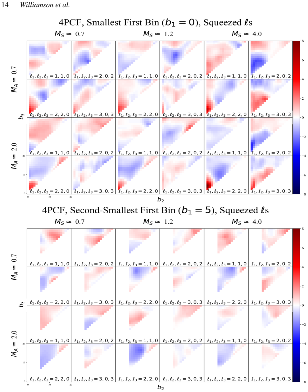
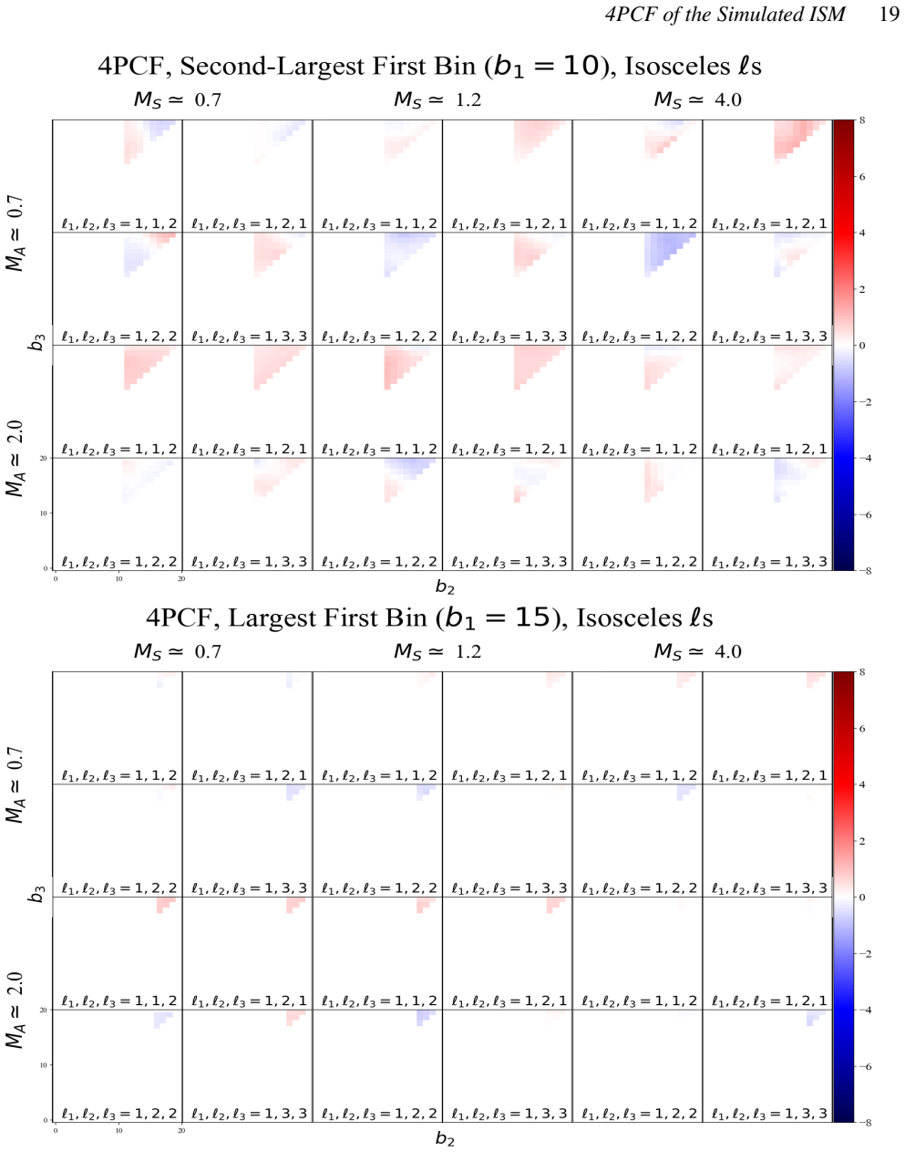
On the paper's own terms, the discovery is that the connected 4PCF of the logarithmic density field in isothermal, non-self-gravitating MHD turbulence is detectable at high signal-to-noise and carries physical information beyond the 2PCF and 3PCF. The 34 measured angular modes respond systematically to the sonic Mach number $M_{\rm S}$, the Alfvénic Mach number $M_{\rm A}$, and the radial bin scales: parity-even modes dominate and are increasingly suppressed as $M_{\rm A}$ grows, while parity-odd modes are fainter but persist, retaining structure at high parameter values. The key physical claim is that these parity-odd modes are generated by a large-scale coherent magnetic field, making the 4PCF a potential test of magnetic-field coherence that does not require measuring polarization.
Load-bearing premise
The load-bearing premise is that the two Alfvénic Mach numbers used (0.7 and 2.0) and the absence of a simulation with the magnetic field turned off are enough to attribute the parity-odd 4PCF modes specifically to a coherent magnetic field; if anisotropic driving, grid resolution, or box-scale effects can also generate them, the central interpretation is not isolated.
Editorial extensions
If this is right
- The connected 4PCF joins the 2PCF and 3PCF as a summary statistic for ISM turbulence, capturing correlations among tetrahedra of density points that lower-order statistics miss.
- Parity-odd 4PCF modes give an observable route to testing whether a magnetic field is coherent over large scales, independent of dust polarization measurements.
- The measured trends with $M_{\rm A}$, $M_{\rm S}$, and radial bins can be used in reverse: given a 4PCF measurement, one could constrain the sonic and Alfvénic Mach numbers of an observed turbulent region.
- Making all 10 Mach-number combinations, 9 time slices, and 34 modes public lets the community test other diagnostics without re-running the simulations.
- Extending the pipeline to projected CO emission maps would yield the first 4PCF study of real ISM data with feedback.
Reading between the lines
- If parity-odd 4PCF amplitudes really track field coherence, then a stacked measurement across many molecular clouds could constrain the coherence scale of galactic magnetic fields without needing to resolve polarization angles.
- Because the simulations use only solenoidal large-scale driving, the parity-odd signal could partly reflect driving symmetry; a test with compressive driving at the same $M_{\rm A}$ would separate driving effects from magnetic-field effects.
- The strong survival of squeezed and scalene parity-odd modes at high $M_{\rm A}$ suggests these configurations are the best targets for noisy observational data, where equilateral modes may be undetectable.
- A Fourier-space analog, the connected trispectrum, should show the same parity-odd signature; comparing the two estimators would cross-check systematics such as binning and the FFT grid.
Signed reviews
Editorial analysis
A structured set of objections, weighed in public.
Referee Report
Summary. The paper presents the first application of the connected 4-point correlation function (4PCF) to magnetohydrodynamic turbulence simulations of the interstellar medium. Using the sarabande code, the authors decompose the 4PCF in an isotropic basis, isolate the connected non-Gaussian component, and measure 34 multipole configurations on 256^3 isothermal, non-self-gravitating CATS simulations with varying sonic and Alfvénic Mach numbers. The main scientific claims are that the connected 4PCF shows rich, parameter-dependent structure that can serve as a future ISM diagnostic, and that a large-scale coherent magnetic field produces parity-odd 4PCF modes. All measured 4PCF coefficients are promised to be made public.
Significance. If the measurement is robust, this is the first 4PCF estimate on MHD turbulence and a genuinely new non-Gaussian summary statistic for ISM studies. The work extends an established 3PCF pipeline, clearly explains the connected-piece subtraction, and releases a large set of measured coefficients, which is a useful community resource. The parity-odd claim, however, is the paper's most novel physical result and is also its least controlled: no null control is presented, the significance normalization is based on only nine time slices, and the symmetry argument for why a uniform magnetic field should produce odd-parity modes is not made. The exploratory and qualitative parts of the paper are sound in spirit, but the central attribution of parity-odd modes to magnetic-field coherence needs substantially stronger support before the abstract-level claim can be accepted.
major comments (3)
- [§2.3, §2.4, §4.6.2, Abstract] The claim that a large-scale coherent magnetic field leads to parity-odd 4PCF modes is not supported by the present analysis. The ideal MHD equations, Eqs. (13)-(15), together with the solenoidal forcing described in §2.4 and no stated helicity injection, are invariant under the parity transformation (v → −v, B → B, ρ unchanged); a uniform background magnetic field is a pseudovector and does not break this invariance. The ensemble-averaged density 4PCF should therefore satisfy ⟨ζ(r1,r2,r3)⟩ = ⟨ζ(−r1,−r2,−r3)⟩, so coefficients with ℓ1+ℓ2+ℓ3 odd should vanish. The manuscript includes no B=0 hydrodynamic run, no phase-randomized Gaussian null, and no test for helical forcing, so the nonzero parity-odd signal in Figs. 7-26 and A1-A10 cannot be attributed to magnetic-field coherence rather than to finite-sample fluctuations or numerical asymmetries. A null test is essential before the abstract statement can stand.
- [§3, Figs. 7-26 and A1-A10] The 'signal-to-noise ratio' is computed by normalizing with the standard deviation across only nine time slices, which are not independent realizations and for which no covariance matrix, jackknife, or bootstrap is provided. With 34 multipole configurations and many radial bins, the appearance of values approaching ±8 under the null is expected purely from multiple testing, and no correction for this is given. The text itself concedes in §5 that covariance testing is needed to 'determine an above null detection', confirming that the detection significance is not yet established. The authors should provide a proper null or covariance treatment, or explicitly relabel the figures as raw fluctuation maps rather than S/N detections.
- [§2.4, §4.2, Abstract] The simulation set is not defined consistently. Section 2.4 lists M_S ≃ 0.7, 1.2, 7.0 and M_A ≃ 0.7, 2.0, which gives six Mach-number combinations, while the Abstract states ten M_S, M_A combinations. Section 4.2 additionally refers to a highest value of M_S = 4.0 that does not appear in §2.4. A table listing each simulation, its exact Mach numbers, and the nine time slices used should be provided; without it, the ten-combination claim and the parameter trends in Section 4 are not reproducible.
minor comments (4)
- [§5 and Fig. 4] The text says that Fig. 4 depicts 'the power spectra and power law fit of the connected 4PCF data', but Fig. 4 shows the density power spectra. The cross-reference and description should be corrected.
- [§2.6] The computing-cost statement reports 45,000+ CPU hours for a single 256^3 cube in about 24 wall hours on a 28-CPU node; 28 × 24 = 672 CPU hours, so the reported CPU-hour figure appears to be an error or requires clarification.
- [Fig. 24 caption] The caption contains a typo: 'parity-odd modes reatin more structure' should read 'retain'.
- [Notation throughout] The Alfvénic Mach number is written as M_A in most of the text but as 'M_a' in the caption of Fig. 10; please standardize the notation.
Circularity Check
No circularity found: the 4PCF measurements are self-contained statistical measurements, with self-citations serving as ordinary tool dependencies rather than load-bearing reductions.
full rationale
The paper's claimed derivation chain is a measurement pipeline, not a derivation in which an output is forced by a fitted input. The connected 4PCF estimator (Eqs. 1-12) follows from standard Gaussian decomposition of the four-point function; the parity classification (E(Λ)=+1/-1 for even/odd ℓ1+ℓ2+ℓ3) is a definitional labeling of the expansion, not a fit. The measurements on CATS MHD simulations (Sec. 2.4) are external inputs, and the 4PCF coefficients are computed rather than tuned to any target. The central interpretive claim—that a coherent magnetic field leads to parity-odd modes—is an empirical attribution from the simulation suite, not an equation-level identity: no parameter was fitted to the parity-odd amplitudes and no model output was constructed from them. The many citations to the authors' own code (sarabande; Sunseri et al. 2022) and basis (Cahn & Slepian 2023) are normal tool dependencies; the paper does not invoke a uniqueness theorem or import an ansatz from those works to force its conclusion. The manuscript itself flags that the covariance/null determination remains to be done ('when tested for covariance can determine an above null detection by eliminating the possibility of noise detection in the data'), and the absence of a B=0 control weakens the statistical support for the magnetic-field attribution, but this is a correctness risk, not circularity. Therefore no circular step is present.
Assumptions & free parameters
free parameters (3)
- Inertial range cutoff k_cut =
1.2e-1
- Multipole truncation lmax =
3
- Number of radial bins =
20
assumptions (4)
- domain assumption The nine time slices of each simulation are treated as independent realizations when computing the signal-to-noise ratio.
- domain assumption The simulations represent ISM conditions despite having no self-gravity, being isothermal, and being driven at a single scale k=2.5.
- standard math Subtracting products of 2PCFs yields the connected, purely non-Gaussian 4PCF.
- domain assumption The log-density normalization in Eq. (16) removes the mean and sets unit variance without biasing the 4PCF.
Cite this review
Pith. "Pith review of First Measurements of the 4-Point Correlation Function of Magnetohydrodynamic Turbulence as a Novel Probe of the Interstellar Medium." pith.science (2026). https://pith.science/paper/EEICALHY
@misc{pith2026241203967,
  author       = {Pith},
  title        = {Pith review of: First Measurements of the 4-Point Correlation Function of Magnetohydrodynamic Turbulence as a Novel Probe of the Interstellar Medium},
  year         = {2026},
  howpublished = {\url{https://pith.science/paper/EEICALHY}},
  note         = {Machine review of arXiv:2412.03967}
}
abstract
In the Interstellar Medium (ISM), gas and dust evolve under magnetohydrodynamic (MHD) turbulence. This produces dense, non-linear structures that then seed star formation. Observationally and theoretically, turbulence is quantified by summary statistics such as the 2-Point Correlation Function (2PCF) or its Fourier-space analog the power spectrum. These cannot capture the non-Gaussian correlations coming from turbulence's highly non-linear nature. We here for the first time apply the 4-Point Correlation Function (4PCF) to turbulence, measuring it on a large suite of MHD simulations that mirror, as well as currently possible, the conditions expected in the ISM. The 4PCF captures the dependence of correlations between quadruplets of density points on the geometry of the tetrahedron they form. Using a novel functionality added to the \textsc{sarabande} code specifically for this work, we isolate the purely non-Gaussian piece of the 4PCF. We then explore simulations with a range of pressures, $P$, and magnetic fields, $B$ (but without self-gravity); these are quantified by different sonic $(M_{\rm S})$ and Alfv\'enic $(M_{\rm A})$ Mach numbers. We show that the 4PCF has rich behavior that can in future be used as a diagnostic of ISM conditions. We also show that a large-scale coherent magnetic field leads to parity-odd modes of the 4PCF, a clean test of magnetic field coherence with observational ramifications. All our measurements of the 4PCF (10 $M_{\rm S}, M_{\rm A}$ combinations, 9 time-slices for each, 34 4PCF modes for each) are made public for the community to explore.
Figures


Figures from the paper (25 more)






Forward citations
Cited by 1 Pith paper
-
Analytic Model for Covariance Matrices of the 2-, 3-, and 4-Point Correlation Functions in the Gaussian Random Field Approximation
Closed-form analytic covariance templates for the 2, 3, and 4 point galaxy correlation functions, built from a 1/k power-law power spectrum, reproduce Boltzmann-code results at percent level and trace sparsity to clos...
Reference graph
Works this paper leans on
-
[1]
write newline
" write newline "" before.all 'output.state := FUNCTION fin.entry write newline FUNCTION new.block output.state before.all = 'skip after.block 'output.state := if FUNCTION new.sentence output.state after.block = 'skip output.state before.all = 'skip after.sentence 'output.state := if if FUNCTION not #0 #1 if FUNCTION and 'skip pop #0 if FUNCTION or pop #1...
-
[2]
N., 2013, Journal of Improbable Astronomy, 1, 1
Author A. N., 2013, Journal of Improbable Astronomy, 1, 1
2013
-
[3]
D., 2015, Journal of Interesting Stuff, 17, 198
Jones C. D., 2015, Journal of Interesting Stuff, 17, 198
2015
-
[4]
B., 2014, The Example Journal, 12, 345 (Paper I)
Smith A. B., 2014, The Example Journal, 12, 345 (Paper I)
2014
-
[5]
Bialy S., Burkhart B., 2020, @doi [The Astrophysical Journal] 10.3847/1538-4357/ab6a82 , 890, 155
-
[6]
Burkhart B., 2009, @doi [The Astrophysical Journal] 10.1088/0004-637X/694/2/1071 , 694, 1071
-
[7]
Burkhart B., Lazarian A., 2011, Statistical Tools of Interstellar Turbulence: Bridging the Gap Between Numerics and Observations ( @eprint arXiv 1105.0929 ), https://arxiv.org/abs/1105.0929
work page Pith review arXiv 2011
-
[8]
M., 2016, @doi [The Astrophysical Journal] 10.3847/0004-637X/827/1/26 , 719, 116
Burkhart B., Lazarian A., Kulsrud R. M., 2016, @doi [The Astrophysical Journal] 10.3847/0004-637X/827/1/26 , 719, 116
Show all 54 references
-
[9]
Burkhart B., et al., 2020, @doi [The Astrophysical Journal] 10.3847/1538-4357/abbd77 , 905, 14
2020 doi
-
[10]
N., Slepian Z., 2023, @doi [Journal of Physics A Mathematical General] 10.1088/1751-8121/acdfc4 , https://ui.adsabs.harvard.edu/abs/2023JPhA...56F5204C 56, 325204
Cahn R. N., Slepian Z., 2023, @doi [Journal of Physics A Mathematical General] 10.1088/1751-8121/acdfc4 , https://ui.adsabs.harvard.edu/abs/2023JPhA...56F5204C 56, 325204
2023 doi
-
[11]
N., Slepian Z., Hou J., 2023, @doi [ ] 10.1103/PhysRevLett.130.201002 , https://ui.adsabs.harvard.edu/abs/2023PhRvL.130t1002C 130, 201002
Cahn R. N., Slepian Z., Hou J., 2023, @doi [ ] 10.1103/PhysRevLett.130.201002 , https://ui.adsabs.harvard.edu/abs/2023PhRvL.130t1002C 130, 201002
2023 doi
-
[12]
Ceverino D., Klypin A., 2009, @doi [The Astrophysical Journal] 10.1088/0004-637X/695/1/292 , 695, 292
2009 doi
-
[13]
Cho J., Lazarian A., 2003, @doi [The Astrophysical Journal] 10.1086/377106 , 595, 812
2003 doi
-
[14]
G., Elmegreen D
Elmegreen B. G., Elmegreen D. M., 1987, @doi [The Astrophysical Journal] 10.1086/165536 , 320, 182
1987 doi
-
[15]
G., Elmegreen D
Elmegreen B. G., Elmegreen D. M., 2001, @doi [The Astronomical Journal] 10.1086/319392 , 121, 1507
2001 doi
-
[16]
G., Scalo J., 2004, @doi [Astrophysical Journal Supplement Series] 10.1086/425652 , 155, 109
Elmegreen B. G., Scalo J., 2004, @doi [Astrophysical Journal Supplement Series] 10.1086/425652 , 155, 109
2004 doi
-
[17]
C.-L., 2014, @doi [The Astrophysical Journal Letters] 10.1088/2041-8205/784/2/L26 , 24, e044005
Falceta-Gonçalves D., Kowal G., Falgarone E., Chian A. C.-L., 2014, @doi [The Astrophysical Journal Letters] 10.1088/2041-8205/784/2/L26 , 24, e044005
2014 doi
-
[18]
S., Schmidt W., 2008, @doi [The Astrophysical Journal] 10.1086/592084 , 688, 1022
Federrath C., Klessen R. S., Schmidt W., 2008, @doi [The Astrophysical Journal] 10.1086/592084 , 688, 1022
2008 doi
-
[19]
S., Schmidt W., 2009, @doi [The Astrophysical Journal] 10.1088/0004-637X/692/1/364 , 692, 364
Federrath C., Klessen R. S., Schmidt W., 2009, @doi [The Astrophysical Journal] 10.1088/0004-637X/692/1/364 , 692, 364
2009 doi
-
[20]
M., 2001, @doi [Reviews of Modern Physics] 10.1103/RevModPhys.73.1031 , 73, 1031
Ferrière K. M., 2001, @doi [Reviews of Modern Physics] 10.1103/RevModPhys.73.1031 , 73, 1031
2001 doi
-
[21]
Friesen M., Slepian Z., et al., 2022, @doi [The Astrophysical Journal Supplement Series] 10.3847/1538-4365/ac4eb0 , 261, 45
2022 doi
-
[22]
Garcia F., Slepian Z., 2021, @doi [The Astrophysical Journal] 10.3847/1538-4357/abf528 , 914, 123
2021 doi
-
[23]
P., Klessen R
Girichidis P., Konstandin L., Whitworth A. P., Klessen R. S., 2014, @doi [The Astrophysical Journal] 10.1088/0004-637X/781/2/91 , 781, 91
2014 doi
-
[24]
M., 2018, PhD thesis, University of Surrey, https://researchportal.surrey.ac.uk/en/publications
Grisdale K. M., 2018, PhD thesis, University of Surrey, https://researchportal.surrey.ac.uk/en/publications
2018
-
[25]
C., Hopkins P
Hayward C. C., Hopkins P. F., 2017, @doi [Monthly Notices of the Royal Astronomical Society] 10.1093/mnras/stw2793 , 465, 1682
2017 doi
- [26]
-
[27]
C., 2017, @doi [The Astrophysical Journal] 10.3847/1538-4357/aa8d96 , 849, 48
Kim C.-G., Ostriker E. C., 2017, @doi [The Astrophysical Journal] 10.3847/1538-4357/aa8d96 , 849, 48
2017 doi
-
[28]
S., 2004, @doi [Reviews of Modern Physics] 10.1103/RevModPhys.76.125 , 76, 125
Mac Low M.-M., Klessen R. S., 2004, @doi [Reviews of Modern Physics] 10.1103/RevModPhys.76.125 , 76, 125
2004 doi
-
[29]
M., 2007, Introductory Lectures on Turbulence: Physics, Mathematics and Modeling
McDonough J. M., 2007, Introductory Lectures on Turbulence: Physics, Mathematics and Modeling. University of Kentucky, https://uknowledge.uky.edu/me_textbooks/2/
2007
-
[30]
F., Ostriker E
McKee C. F., Ostriker E. C., 2007, @doi [ ] 10.1146/annurev.astro.45.051806.110602 , https://ui.adsabs.harvard.edu/abs/2007ARA&A..45..565M 45, 565
2007 arXiv
-
[31]
E., et al., 2022, @doi [ ] 10.1093/mnras/stac508 , https://ui.adsabs.harvard.edu/abs/2022MNRAS.512.1196M 512, 1196
Miller A. E., et al., 2022, @doi [ ] 10.1093/mnras/stac508 , https://ui.adsabs.harvard.edu/abs/2022MNRAS.512.1196M 512, 1196
2022 doi
-
[32]
Motte F., Bontemps S., Louvet F., 2021, @doi [Annual Review of Astronomy and Astrophysics] 10.1146/annurev-astro-032620-021945 , 59, 143
2021 doi
-
[33]
J., Burkhart B., Shelley M
O'Brien M. J., Burkhart B., Shelley M. J., 2022, @doi [The Astrophysical Journal] 10.3847/1538-4357/ac6502 , 930, 149
2022 doi
- [34]
-
[35]
C., Stone J
Ostriker E. C., Stone J. M., Gammie C. F., 2001, @doi [The Astrophysical Journal] 10.1086/318290 , 546, 980
2001 doi
-
[36]
Padoan P., Nordlund A., 1999, @doi [The Astrophysical Journal] 10.1086/307984 , 526, 279
1999 doi
-
[37]
Philcox O. H. E., Slepian Z., 2022, @doi [Physical Review D] 10.1103/PhysRevD.106.063514 , 106, 063514
2022 doi
- [38]
-
[39]
Philcox O. H. E., Cahn A., Slepian Z., 2022, @doi [Monthly Notices of the Royal Astronomical Society] 10.1093/mnras/stac366 , 511, 5347
2022 doi
-
[40]
Portillo S. K. N., Slepian Z., Burkhart B., Kahraman S., Finkbeiner D. P., 2018, @doi [ ] 10.3847/1538-4357/aacb80 , https://ui.adsabs.harvard.edu/abs/2018ApJ...862..119P 862, 119
2018 doi
-
[41]
Riaz R., Schleicher D. R. G., Vanaverbeke S., Klessen R. S., Saavedra-Bastidas J., 2024, @doi [Monthly Notices of the Royal Astronomical Society] 10.1093/mnras/stae1451 , 532, 763
2024 doi
-
[42]
Slepian Z., 2024, @doi [RAS Techniques and Instruments] 10.1093/rasti/rzae028 , 3, 584
2024 doi
-
[43]
J., 2015, @doi [ ] 10.1093/mnras/stv2119 , https://ui.adsabs.harvard.edu/abs/2015MNRAS.454.4142S 454, 4142
Slepian Z., Eisenstein D. J., 2015, @doi [ ] 10.1093/mnras/stv2119 , https://ui.adsabs.harvard.edu/abs/2015MNRAS.454.4142S 454, 4142
2015 doi
-
[44]
J., 2016, @doi [ ] 10.1093/mnrasl/slv133 , https://ui.adsabs.harvard.edu/abs/2016MNRAS.455L..31S 455, L31
Slepian Z., Eisenstein D. J., 2016, @doi [ ] 10.1093/mnrasl/slv133 , https://ui.adsabs.harvard.edu/abs/2016MNRAS.455L..31S 455, L31
2016 doi
-
[45]
J., 2017, @doi [ ] 10.1093/mnras/stx490 , https://ui.adsabs.harvard.edu/abs/2017MNRAS.469.2059S 469, 2059
Slepian Z., Eisenstein D. J., 2017, @doi [ ] 10.1093/mnras/stx490 , https://ui.adsabs.harvard.edu/abs/2017MNRAS.469.2059S 469, 2059
2017 doi
-
[46]
J., 2020, @doi [The Astrophysical Journal] 10.3847/1538-4357/ab7d58 , 892, 116
Slepian Z., Eisenstein D. J., 2020, @doi [The Astrophysical Journal] 10.3847/1538-4357/ab7d58 , 892, 116
2020 doi
-
[47]
Slepian Z., et al., 2017a, @doi [Physical Review D] 10.1103/PhysRevD.95.083520 , 95, 083520
-
[48]
Slepian Z., et al., 2017b, @doi [The Astrophysical Journal] 10.3847/1538-4357/835/1/71 , 835, 71
-
[49]
Slepian Z., et al., 2018, @doi [The Astrophysical Journal] 10.3847/1538-4357/aad1a9 , 864, 128
2018 doi
- [50]
-
[51]
P., 2022, @doi [arXiv e-prints] 10.48550/arXiv.2210.10206 , https://ui.adsabs.harvard.edu/abs/2022arXiv221010206S p
Sunseri J., Slepian Z., Portillo S., Hou J., Kahraman S., Finkbeiner D. P., 2022, @doi [arXiv e-prints] 10.48550/arXiv.2210.10206 , https://ui.adsabs.harvard.edu/abs/2022arXiv221010206S p. arXiv:2210.10206
-
[52]
Vázquez-Semadeni E., 1994, @doi [The Astrophysical Journal] 10.1086/173652 , 423, 681
1994 doi
-
[53]
327, The Initial Mass Function 50 Years Later
Vázquez-Semadeni E., 2005, in Corbelli E., Palla F., Zinnecker H., eds, Astrophysics and Space Science Library, Vol. 327, The Initial Mass Function 50 Years Later. Springer, pp 371--378, @doi 10.1007/978-1-4020-3407-7_70 , https://arxiv.org/abs/astro-ph/0409553
2005 arXiv
-
[54]
A., 2005, @doi [Journal of Physics: Conference Series] 10.1088/1742-6596/6/1/001 , 6, 1
Williams D. A., 2005, @doi [Journal of Physics: Conference Series] 10.1088/1742-6596/6/1/001 , 6, 1
2005 doi
Reviewed August 11, 2026 · model on record in the stance chip above.
Discussion (0). Continue with ORCID to comment.