REVIEW 2 major objections 4 minor 1 cited by
Rapid Bayesian Seismic Tomography using Graph Mixture Density Networks
T0 review · 2 major / 4 minor · reviewed 2026-08-11 · deepseek-v4-flash
Pith's one-line read This paper claims that a single trained graph mixture density network can deliver posterior mean and uncertainty maps for seismic travel-time tomography in about 0.6 seconds, matching Markov chain Monte Carlo quality even when the number…
desk verdict A useful graph-MDN extension for variable-size tomography, but the 'accurate' claim outruns the evidence: validation is visual only and the paper's own uncertainty mismatch is unquantified. read the letter →
The pith
A machine-rendered reading of the paper's core claim, the machinery that carries it, and where it could break.
The reading
What carries the argument
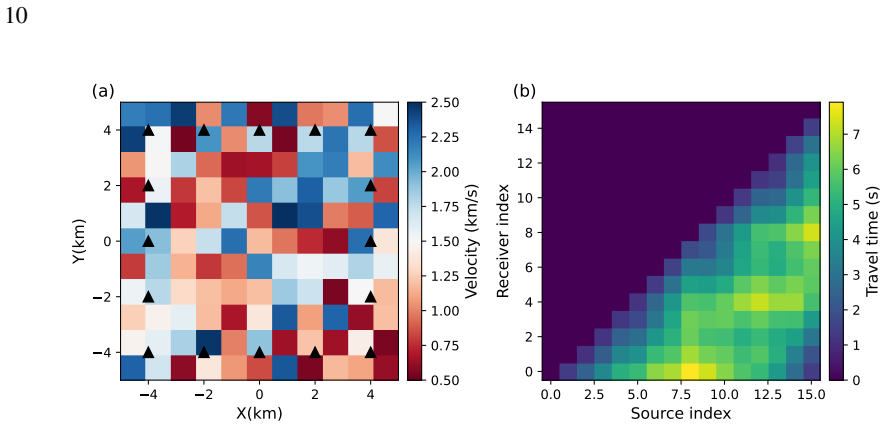
The central object is the graph mixture density network, a neural network that takes a graph as input and outputs the parameters of a Gaussian mixture model approximating the posterior probability density p(m|d). Travel-time data are encoded as a graph: stations are nodes with coordinate features, and each station pair with a measured travel time becomes an undirected edge whose feature is the path-averaged velocity derived from the travel time and inter-station distance. The network stacks graph transformer layers, which aggregate node and edge features through attention coefficients, with graph linear layers; the updated node features are pooled by a global mean, and a final linear layer emits the mixture coefficients, means, and diagonal standard deviations of ten Gaussian kernels. During training, station-pair edges are randomly dropped at each iteration (rate 0.1 in the synthetic case, 0.6 for the real data), teaching the network to handle variable data sizes. The load-bearing identity is the graph representation itself: because predictions depend only on graph structure, the same trained network applies to any subset of the available station pairs.
What would settle it
Run the same graph MDN on a tomographic problem with a larger model dimension, such as a 3D grid or a 2D grid with more than 100 cells, and compare posterior statistics against a converged McMC or Hamiltonian Monte Carlo reference; if the standard-deviation maps diverge systematically or the network cannot represent correlations between neighboring cells, the claim of accurate rapid Bayesian tomography fails. A cheaper discriminating test is to train on data with strongly multimodal posteriors or with correlated model parameters and check whether the diagonal-Gaussian mixture reproduces the reference covariance.
Extended reading notes
Core claim
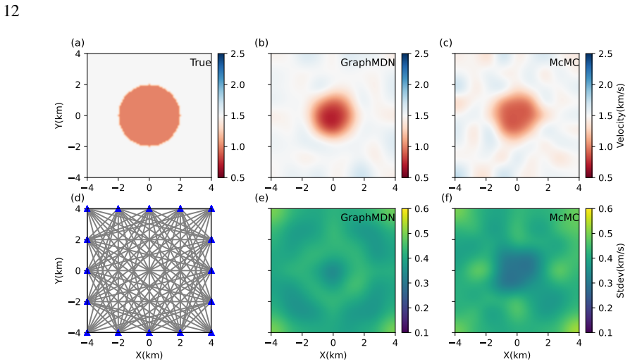
The central claim is that the graph MDN removes the fixed-input limitation of neural-network-based Bayesian inversion: because the network operates on a graph rather than a fixed-length vector, it can ingest any subset of station pairs and still output an approximate posterior pdf over the velocity model. The validation uses 200,000 simulated velocity models whose travel times were computed with the fast marching method, then compares the network's posterior mean and standard deviation maps against adaptive Metropolis-Hastings McMC runs of six chains of one million samples each. On the synthetic problem (81 model parameters, 16 receivers, full and randomly thinned data), both methods recover the same central low-velocity anomaly, show similar edge effects, and place higher uncertainty where ray coverage is poor. On the real data (six periods, 90 model parameters), the graph MDN reproduces the known geological features of South England and follows the McMC uncertainty pattern, although the magnitudes of the uncertainties differ because MDNs become difficult to train accurately in high dimensions. The paper's conclusion is that for problems requiring many similar tomographic inversions with different numbers of data, a trained graph MDN provides accurate posterior estimates in seconds.
Load-bearing premise
Everything rests on the assumption that a mixture of ten Gaussian kernels with no inter-parameter covariance can faithfully represent a posterior in an 81- or 90-dimensional model space; if that approximation is too crude, the uncertainty maps are biased and the agreement with McMC will not survive harder or higher-dimensional problems.
Editorial extensions
If this is right
- After training, a graph MDN answers a new tomographic problem in about 0.6 seconds, making near-real-time subsurface monitoring and time-lapse imaging feasible for problems that previously required 16 to 21 hours of McMC computation per data set.
- The same trained network can be applied to data sets with different numbers of station pairs, so missing or noisy measurements do not require retraining or a new inversion.
- The graph abstraction carries over to other geophysical inverse problems in which data are organized as pairs of stations or sources and receivers, such as body-wave travel-time tomography.
- When many inversions are needed (for example, one per period or per time window), the one-time training cost is amortized and the method becomes more efficient than running McMC for every data set.
Reading between the lines
- Editorial inference: the architecture suggests a route toward a single array-wide tomographic network trained once on random station subsets and then used for any data availability pattern, including station additions; the paper notes this possibility but does not demonstrate it.
- Editorial inference: the same graph encoding could be applied to other network-based inverse problems with pairwise measurements, such as electrical resistivity or hydrological tomography, provided a forward simulator exists to generate training pairs.
- Editorial inference: the reported agreement is limited to posterior means and standard deviations; the paper does not test whether the full posterior shape, including multimodality or correlations between distant cells, is captured, so the phrase 'comparable posterior pdfs' should be read as applying to these statistics.
- Editorial inference: a natural stress test would increase the number of Gaussian kernels or replace the mixture with a graph-based normalizing flow and measure how the agreement with McMC changes as model dimension grows; the paper itself names invertible neural networks as a possible improvement.
Signed reviews
Editorial analysis
A structured set of objections, weighed in public.
Referee Report
Summary. The paper proposes graph mixture density networks (graph MDNs) for Bayesian seismic travel-time tomography with variable numbers of travel-time data. Travel-time observations between station pairs are represented as a graph, and a graph transformer with edge features feeds a mixture-density-network head that outputs a Gaussian mixture approximation to the posterior over a fixed grid of velocity parameters. The method is demonstrated on a synthetic 2D travel-time tomography problem with 16 receivers and a 9×9 velocity grid, where the number of station pairs is randomly reduced, and on a real Love-wave group-velocity tomography study in South England at six periods with data of varying size. In both cases the posterior means and standard deviations are compared visually with McMC reference solutions, and computational timings are reported. The authors conclude that graph MDNs provide accurate and rapid posterior approximations for variable data sizes.
Significance. If the claims were fully substantiated, the method would be a useful contribution: it removes the fixed-input-size restriction of standard MDNs by using graph neural networks, and it reports orders-of-magnitude speedups after training. The explicit graph representation of station pairs, the edge-dropping training strategy, and the demonstration on both synthetic and real data are strengths. The paper also provides clear network configurations and runtime figures. However, the central claim of 'accurate' posterior approximation is not supported by quantitative validation: the comparison with McMC is visual only, and the paper itself reports that graph-MDN uncertainties are systematically larger than McMC's. The significance therefore depends on whether the authors can supply calibration or coverage metrics and address the expressiveness limitation of a 10-kernel diagonal Gaussian mixture in 81–90 dimensions.
major comments (2)
- [§3 and §4, Figs 4–7 and 10–11] The conclusion that graph MDNs provide comparable posterior pdfs to McMC is based entirely on qualitative visual comparison of posterior mean and standard deviation maps. No quantitative metric (e.g., per-cell mean or standard-deviation error, empirical coverage of the McMC marginals by the MDN predictive intervals, or a divergence measure such as KL) is reported. This matters because the paper notes in §3 that high-standard-deviation features present in the McMC maps (e.g., the four lobes around the central anomaly in Figs 4f and 5f) are not clearly visible in the graph-MDN maps, and in §4 the McMC standard deviations are 'generally smaller than that obtained using graph MDN' (p. 22). A systematic overestimation of variance is not a benign discrepancy: it changes the interpretation of the posterior. I would ask the authors to add quantitative agreement metrics between the graph-MDN and McMC posteriors, and also to report the test-set negative log-likelihood or calibration of the predictive distribution on the held-out 10% of training pairs.
- [§2.2, Eq. (3); §5, first paragraph] The load-bearing approximation is that a mixture of 10 Gaussian kernels with diagonal covariances, Eq. (3), is sufficiently expressive and trainable to represent the posterior in an 81- or 90-dimensional model space. The paper cites universal approximation properties of mixture models, but that is an asymptotic statement. The authors explicitly concede in §5 that 'results obtained using graph MDNs show higher uncertainty estimates than those obtained using McMC because of difficulties of training MDNs in high dimensionality.' That admission directly undercuts the accuracy claim, because an inflated covariance is not an accurate posterior. I would like to see a discussion or demonstration that the chosen number of components and the training budget are adequate: for example, a sensitivity test with more than 10 kernels, a comparison on a lower-dimensional problem where exact posteriors are known, or diagnostics (posterior predictive checks, coverage probabilities) that show the approximation error is acceptable. Without this, the claim in §6 that graph MDNs 'provide accurate approximations of posterior pdfs' is not justified.
minor comments (4)
- [§2.3] The phrase 'We use ReLU activate functions for each graph transformer layer or linear layer' should read 'We use ReLU activation functions for each graph transformer layer or linear layer'.
- [References] The reference to Kingma & Welling (2013) contains a typo: 'Auto-encoding variational Byes' should be 'Auto-encoding variational Bayes'.
- [§3 and §4, timing comparisons] The reported inference times of 0.6 s per data set should clarify whether this figure includes graph construction and data pre-processing or only the network evaluation; this would make the cost comparison with McMC more transparent.
- [§5 vs. §6] The paper only varies the number of station pairs in the experiments, not the number of stations; although §5 discusses training with variable station distributions as a possibility, no experiment demonstrates that scenario, so the broad 'variable sizes of data' phrasing in §6 is stronger than what is shown.
Circularity Check
No significant circularity: the graph MDN is trained on prior-forward samples and benchmarked against independent McMC; the paper's self-citations are contextual and not load-bearing.
full rationale
The derivation chain is not circular. The network is trained on (model, data) pairs drawn from the prior p(m) and the forward likelihood p(d|m), minimizing the negative log likelihood of Eq. (2); this is a standard supervised-learning construction of the conditional p(m|d), with no parameter fitted to the McMC posterior and then renamed a prediction. The McMC comparison is an independent, same-likelihood consistency check rather than an input to training. The paper's admitted limitations (higher uncertainty estimates due to MDN training difficulties in high dimensions; features in McMC not clearly observed in graph MDN; 'the two solutions can have different detailed structures') weaken the accuracy claim but do not reduce any equation to itself. Self-citations such as Zhang & Curtis (2021) are used for problem setup, comparison, and as a citation for the known high-dimensionality limitation of MDNs; they are not invoked as a uniqueness theorem or as the sole justification of the central claim. The graph transformer architecture is cited from an external source (Shi et al. 2020). Consequently, no self-definitional, fitted-input, or self-citation-chain circularity is present.
Assumptions & free parameters
free parameters (5)
- Number of Gaussian mixture components =
10
- Edge drop rate during training =
0.1 (synthetic), 0.6 (real)
- Noise standard deviation (synthetic) =
0.05 s
- Prior bounds =
0.5-2.5 km/s (synthetic), 1.8-4.0 km/s (real)
- Architecture hyperparameters (layers, hidden units, learning rate, iterations) =
e.g., 4 transformer layers, 10 kernels, lr 0.0001, 500 iterations
assumptions (6)
- standard math Bayes' theorem provides the correct posterior for the stated likelihood and prior.
- domain assumption The fast marching method accurately computes travel times for the 2D models.
- domain assumption Data errors are Gaussian with known standard deviation and independent across stations.
- domain assumption Velocity parameters are independent with uniform priors.
- ad hoc to paper A mixture of 10 Gaussian kernels with diagonal covariances can approximate the posterior sufficiently well.
- ad hoc to paper A halo of random cells around the receiver array prevents artificial boundary effects.
Cite this review
Pith. "Pith review of Rapid Bayesian Seismic Tomography using Graph Mixture Density Networks." pith.science (2026). https://pith.science/paper/HSGWGCIY
@misc{pith2026241208080,
  author       = {Pith},
  title        = {Pith review of: Rapid Bayesian Seismic Tomography using Graph Mixture Density Networks},
  year         = {2026},
  howpublished = {\url{https://pith.science/paper/HSGWGCIY}},
  note         = {Machine review of arXiv:2412.08080}
}
read the original abstract
Seismic tomography is a methodology to image subsurface properties of the Earth. In order to better interpret the resulting images, it is important to assess uncertainty in the results. Mixture density networks (MDNs) provide an efficient way to estimate Bayesian posterior probability density functions (pdfs) that describe the uncertainty of tomographic images. However, the method can only be applied in cases where the number of data is fixed, and consequently a large number of practical applications that have variable data sizes cannot be solved. To resolve this issue, we introduce graph neural networks (GNNs) to solve seismic tomographic problems. Graphs are data structure which provides flexible representation of complex, variable systems. GNNs are neural networks that manipulates graph data, and can be combined with MDNs (called graph MDNs) to provide efficient estimates of posterior pdfs for graph data. In this study we apply graph MDNs to seismic tomography by representing travel time data with a graph. We demonstrate the method using both synthetic and real data, and compare the results with those obtained using Markov chain Monte Carlo (McMC). The results show that graph MDNs can provide comparable posterior pdfs to those obtained using McMC at significantly lower cost. We thus conclude that graph MDNs can be used in a range of practical applications that require many similar seismic tomographic problems with different number of data to be solved.
Figures


Figures from the paper (8 more)


Forward citations
Cited by 1 Pith paper
-
Solving All Seismic Tomographic Problems using Deep Learning
A single graph mixture density network trained on random 2D velocity models and station layouts can produce posterior velocity maps for synthetic and real seismic datasets of different sizes and scales.
Reference graph
Works this paper leans on
-
[7]
Auto-encoding variational Byes, arXiv preprint arXiv:1312.6114. Kipf, T. N. & Welling, M.,
-
[11]
Faster Uncertainty Quantification for Inverse Problems with Conditional Normalizing Flows
Faster uncertainty quantification for inverse problems with conditional normalizing flows, arXiv preprint arXiv:2007.07985. Sun, J., Innanen, K., Zhang, T., & Trad, D.,
work page Pith review arXiv 2007
-
[1999]
Regularisation of mixture density networks, in 1999 Ninth Interna- tional Conference on Artificial Neural Networks ICANN 99.(Conf. Publ. No
work page 1999
-
[2000]
A Monte Carlo method to quantify uncertainty in the inversion of zero-offset VSP data, in 2000 SEG Annual Meeting, Society of Exploration Geophysicists. McLachlan, G. J. & Basford, K. E.,
work page 2000
-
[2009]
Real time monitoring of relative velocity changes using ambient seismic noise at the piton de la fournaise volcano (la réunion) from january 2006 to june 2007,Journal of Volcanology and Geothermal Research, 184(1-2), 164–173. Dziewonski, A. M. & Woodhouse, J. H.,
work page 2006
-
[2013]
Spectral networks and locally connected networks on graphs, arXiv preprint arXiv:1312.6203. Burdick, S. & Leki´c, V .,
- [2014]
-
[2016]
Laloy, E., Hérault, R., Lee, J., Jacques, D., & Linde, N.,
Semi-supervised classification with graph convolutional networks,arXiv preprint arXiv:1609.02907. Laloy, E., Hérault, R., Lee, J., Jacques, D., & Linde, N.,
Show all 12 references
-
[2017]
Wu, S., Huang, Q., & Zhao, L.,
Graph attention networks, arXiv preprint arXiv:1710.10903. Wu, S., Huang, Q., & Zhao, L.,
-
[2018]
Arrowsmith, S
Analyzing inverse problems with invertible neural networks, arXiv preprint arXiv:1808.04730. Arrowsmith, S. J., Trugman, D. T., MacCarthy, J., Bergen, K. J., Lumley, D., & Magnani, M. B.,
-
[2019]
2090–2096, IEEE
Multimodal trajectory predictions for autonomous driving using deep convolutional networks, in 2019 International Conference on Robotics and Automation (ICRA), pp. 2090–2096, IEEE. Curtis, A. & Lomax, A.,
2019
-
[2020]
Siahkoohi, A., Rizzuti, G., Witte, P
Masked label prediction: Unified message passing model for semi-supervised classification, arXiv preprint arXiv:2009.03509. Siahkoohi, A., Rizzuti, G., Witte, P. A., & Herrmann, F. J.,
2009 arXiv
Reviewed August 11, 2026 · model on record in the stance chip above.
Discussion (0). Continue with ORCID to comment.