REVIEW 3 major objections 5 minor 63 references
Efficient Bayesian inversion for simultaneous estimation of geometry and spatial field using the Karhunen-Lo\`eve expansion
T0 review · 3 major / 5 minor · reviewed 2026-08-11 · deepseek-v4-flash
Pith's one-line read One Karhunen-Loève solve on a fixed bounding domain is enough for simultaneous estimation of an evolving geometry and its spatial field, cutting the K-L gradient cost from cubic to linear in the mesh size.
desk verdict A genuine computational improvement for K-L-based simultaneous geometry and field inversion, with one under-tested truncation approximation that needs a 2D baseline. read the letter →
The pith
A machine-rendered reading of the paper's core claim, the machinery that carries it, and where it could break.
The reading
What carries the argument
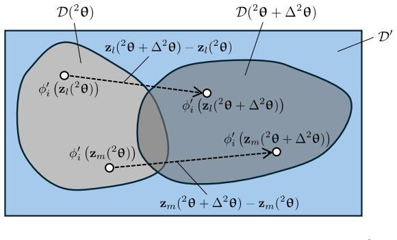
The load-bearing object is the domain independence property of the K-L expansion: for two overlapping domains $D$ and $D'$, the complete K-L expansions built on each domain have the same first and second moments at all points in the overlap, even though the individual eigenpairs differ. The paper exploits this by choosing a bounding domain $D'$ and solving the integral eigenvalue problem once by the Nyström method, then treating the eigenfunctions as fixed shapes whose values at the moving points $z_l(2\theta)$ change only through the geometry-dependent coordinates. The gradient machinery is then Eqs. (46)-(48): the derivative with respect to the field coefficients is the fixed eigenpair term $\sqrt{\lambda'_i}\phi'_i(z(2\theta))$, and the derivative with respect to the geometry parameters is a sum over the already computed eigenpairs times $\partial\phi'_i/\partial 2\theta$, which Eq. (48) reduces to a weighted sum of derivatives of the Gaussian autocovariance kernel. This avoids both repeated eigenvalue solves and pseudo-inverse computations, leaving a per-element cost that is independent of the mesh size.
What would settle it
Take a 2D problem with a small cavity whose radius is comparable to the prior correlation length, run the proposed fixed-bounding-domain inversion and a reference inversion that recomputes the integral eigenvalue problem on each updated domain, and compare the posterior distributions of the cavity center and radius: if the 95% credible intervals for any geometry parameter differ by more than the width of the reference interval, or if the posterior mean of the conductivity field deviates systematically near the boundary, the domain-independence truncation error is not negligible for that configuration.
Extended reading notes
Core claim
The central claim is that the K-L expansion constructed on any fixed bounding domain $D'$ that contains every visited domain $D(2\theta)$ can stand in for the domain-dependent expansion on each $D(2\theta)$ during inversion. Because the autocovariance function is the same on the overlap, the first- and second-order moments of the corresponding random fields coincide on $D(2\theta)$, so the truncated field $\hat u(z,{}^1\theta) = \bar u(z)+\sum_{i=1}^{M_1}\sqrt{\lambda'_i}\phi'_i(z)\,{}^1\theta_i$ remains a valid representation as the geometry parameters $2\theta$ move the evaluation points. The gradient formulas (46)-(48) express the spatial-field derivative directly as $\sqrt{\lambda'_i}\phi'_i(z(2\theta))$ and the geometry derivative through $\partial C(z(2\theta),z'_j)/\partial 2\theta$, quantities available from the single Nyström solve on $D'$, eliminating the repeated eigenvalue solves and the Moore-Penrose inverse required by the earlier discrete-K-L method. The paper demonstrates in a 1D three-layer seepage problem that the proposed scheme yields posteriors almost identical to the earlier simultaneous method while reducing the K-L gradient complexity from $O(n_e^3)$ to $O(n_e)$, and in 1D and 2D seepage problems that it identifies the interface location and its uncertainty more accurately than spatial-field-only estimation.
Load-bearing premise
The assumption that carries the method is that the truncated K-L expansion computed once on the fixed bounding domain still represents the random field accurately on every updated subdomain visited during sampling; the paper notes the truncation error is larger for the bounding-domain expansion and verifies it is negligible only in the 1D comparison.
Editorial extensions
If this is right
- For any inverse problem where a bounding domain can enclose all geometry realizations, the K-L gradient is no longer the computational bottleneck: its cost per HMC leapfrog step is $O(n_e)$ rather than $O(n_e^3)$.
- Simultaneous estimation of the interface and the field needs fewer unknown parameters than field-only inversion, because the boundary parameterization carries the discontinuity and the prior correlation length can be larger.
- The posterior for the boundary location and the conductivity field can be reported together, with boundary uncertainty expressed as highest-posterior-density regions that envelop the true interface in the tested 1D and 2D seepage problems.
- The method preserves the posterior accuracy of the earlier simultaneous method; the truncation error introduced by using the bounding-domain expansion had a negligible effect on the 1D inversion results.
- Because the forward solve remains the dominant cost, applying the method to higher-dimensional or transient problems depends mainly on the forward solver's scaling rather than on the K-L gradient computation.
Reading between the lines
- The same fixed-eigenpair gradient strategy should carry over to level-set or immersed-boundary parameterizations, because the field representation itself never depends on the evolving domain once the bounding-domain eigenpairs are fixed.
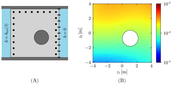
- A direct test of the truncation-error assumption would be to repeat the 2D cavity experiment with a solver that recomputes the IEVP on each updated domain; the paper does not include that comparison in 2D.
- If the correlation length is inferred during inversion, a parameterized K-L expansion or a nested eigenvalue solve on the bounding domain would be needed, because the IEVP changes with the correlation length.
- The reported asymptotic gain is for the K-L gradient only; in large 2D and 3D problems the forward solver's linear-algebra cost will typically determine whether the overall speedup approaches two orders of magnitude.
Editorial analysis
A structured set of objections, weighed in public.
Referee Report
Summary. The paper develops an efficient Bayesian inversion method for simultaneous estimation of spatial random fields and geometric parameters. The key idea is to exploit the domain independence property of the Karhunen-Loève expansion: the integral eigenvalue problem (IEVP) is solved once on a fixed bounding domain D′ that contains all possible updated domains D(2θ), and the resulting eigenpairs are reused throughout Hamiltonian Monte Carlo sampling. This avoids repeated IEVP solves and eliminates the Moore-Penrose inverse computations needed for shape derivatives in the prior discrete-K-L method of Koch et al. (2021). Gradient formulas for the K-L expansion w.r.t. geometry parameters are derived (Eqs. (46)–(48)) with O(ne) complexity. The method is tested on 1D and 2D steady seepage problems, showing gains in computation time and comparable posterior estimates to the baseline in the 1D case.
Significance. If the central approximation is justified, the paper offers a practically useful computational speedup: the K-L gradient cost is reduced from O(ne^3) to O(ne), and the implementation avoids pseudoinverse computations. The 1D comparison shows that the proposed method can reproduce the discrete-K-L simultaneous inversion results almost exactly, while running much faster. The exposition is clear, and the gradient derivation is internally consistent. The main caveat is that the load-bearing approximation—using a truncated K-L expansion on the bounding domain for all updated subdomains—is not quantitatively controlled, and the 2D demonstration does not compare against the discrete-K-L baseline. Thus the significance is conditional: the method is promising, but the evidence for its central claim is incomplete.
major comments (3)
- [§2.2 and §5.2] The central approximation of the paper is that a truncated K-L expansion computed on a fixed bounding domain D′ accurately represents the random field on every updated domain D(2θ). Section 2.2 concedes that the domain independence property holds for the complete expansion and that truncation introduces an error, which is larger for the bounding-domain expansion. However, no quantitative error bound is provided, and the only empirical support is the 1D comparison in Section 5.1.1. The 2D study in Section 5.2 contains no comparison against the discrete-K-L simultaneous method, so the equivalence claim is unverified in the setting where the efficiency gain matters most. I would like to see either a rigorous truncation-error estimate in terms of the eigenvalue decay and the geometry of D(2θ), or a 2D baseline comparison, before the central claim can be accepted.
- [§2.3 and Eq. (12)] The text states that 'due to the domain independence property, the K-L expansion of u constructed on D′ is equivalent to that on D(2θ)'. This is only true for the complete expansion. The truncated expansion in Eq. (12) induces a prior covariance on D(2θ) given by Σ_{i≤M1} λ′_i φ′_i(z)φ′_i(z∗), which is not the optimal M1-term truncated K-L covariance on D(2θ). The authors should explicitly label this as an approximation and quantify its effect on posterior inference, for example by reporting the captured variance fraction on the actual subdomains for the tested cases, not just on D′.
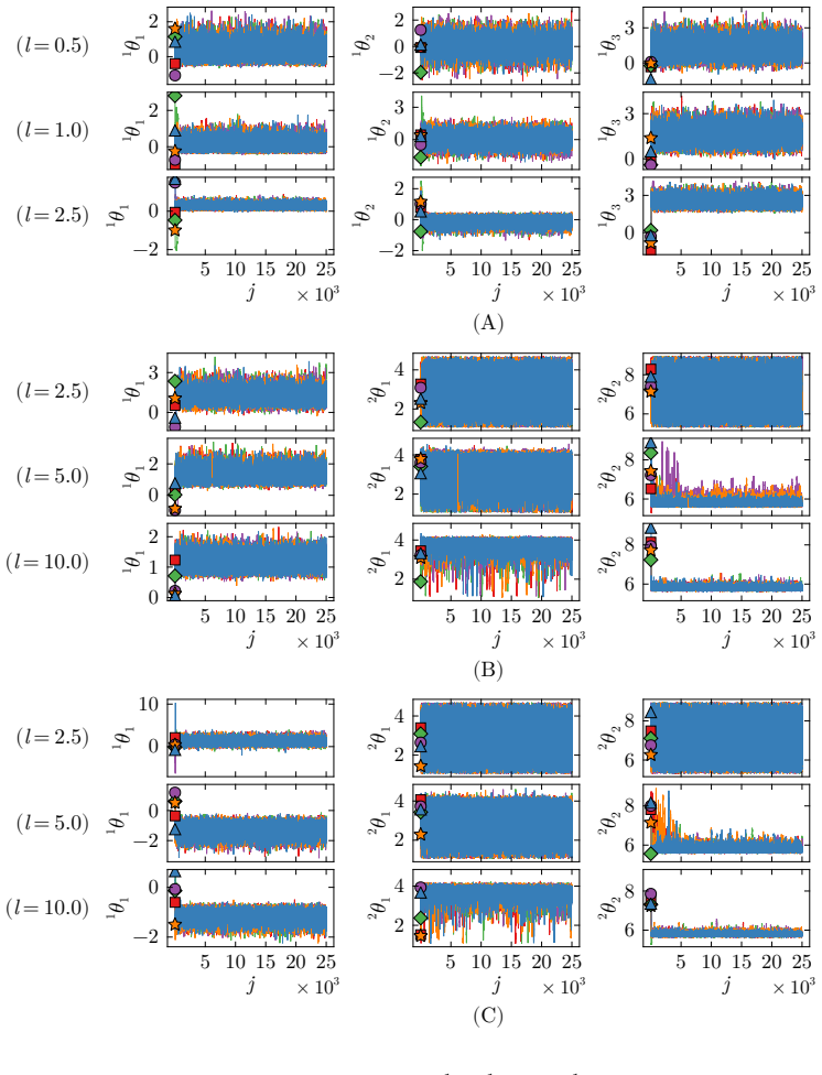
- [§5.1.1 and Table 1] The comparison with Koch et al. (2021) uses different numbers of K-L terms for the two simultaneous methods (e.g., M=16 vs. M=13 for l=2.5 m). The truncation threshold λ>10^-3 is applied on different domains (D′ for the proposed method, D1 and D2 for the baseline), so the amount of captured variance per domain may differ. To substantiate the claim that the truncation error has negligible effect on the inversion results, the authors should report the variance fraction captured on D(2θ) for each method and perhaps a quantitative posterior discrepancy measure (e.g., Wasserstein distance between marginal posteriors) rather than only visual comparison of mean and credible intervals.
minor comments (5)
- [Eq. (4)] There is a typo in the truncated K-L expansion: the right-hand side should involve the mean function X̄(z) (or u(z)), not X(z,ω) itself. As written, the equation is circular.
- [Eq. (12) and Section 2.4] The notation u(z,ω) = u(z,1θ(ω)) is confusing because u is used both for the random field and for the mean function. Please use a clearer notation, for example u(z,1θ) for the random field and ū(z) for its mean.
- [Introduction, reference [5]] The spatial-field-only estimation method is cited as [5], which is a paper on elastic modulus estimation. Since the numerical examples are seepage flow problems, the authors should cite a more directly relevant spatial-field-only inversion method, or clarify that [5] is used as a general adjoint-HMC framework.
- [Section 4, Eqs. (43)–(44)] The shape derivative formulas for G and |J_e| are stated without derivation or reference to the exact finite element formulation. While they are plausible and follow [33], a brief explanation of the notation (e.g., the meaning of G as the matrix of global shape-function derivatives) would improve readability.
- [Section 5.1.2, Fig. 9] The two-orders-of-magnitude improvement is measured for the K-L gradient computation time at a specific parameter setting. It would be helpful to state the wall-clock times or the hardware used, so that the reader can gauge the practical impact.
Circularity Check
No significant circularity: the central claim rests on an external domain-independence property and is benchmarked against a distinct discrete-K-L method; the acknowledged truncation error is a validation concern, not a circular reduction.
full rationale
The derivation chain is self-contained. The fixed-bounding-domain IEVP construction (Sec. 2.2, Eqs. (6)-(9)) is the external domain-independence property of Pranesh and Ghosh (2015); the paper does not define the target result in terms of the method's own output. The gradient formulas (46)-(48) follow algebraically from the truncated expansion (12) and the Nystrom interpolation (18), with no fitted parameter relabeled as a prediction. The comparison in Sec. 5.1.1 against Koch et al. (2021) is a genuine independent baseline: that method uses the discrete K-L expansion and Moore-Penrose shape derivatives (Appendix A), so the near-identical posteriors are evidence, not construction. The only caveat is the truncation error acknowledged in Sec. 2.2 ('an error is introduced when the truncated K-L expansions ... are used') and asserted negligible in Sec. 5.1.1 from 1D results only; the 2D demonstration contains no baseline comparison. This is a validation gap or correctness risk, not a circularity: no equation of the proposed method reduces to the baseline result or to its own assumptions by definition.
Assumptions & free parameters
free parameters (5)
- K-L truncation threshold =
10^-3 (1D); λmax × 10^-3 (2D)
- Prior correlation length l =
Varied across experiments: 0.5, 1, 2.5; 2.5, 5, 10; 2, 4; 4, 8 m
- Hydraulic conductivity lower bound kmin =
10^-7 m/s
- Mesh stiffness parameters =
χ = 1, J0 = 1, Young's modulus = 2500 MPa, Poisson's ratio = 0.25
- Geometry prior mean and covariance =
1D: N([2.5, 7.5], I2) truncated; 2D: N([0, 0, 0.5], I3) truncated
assumptions (7)
- standard math Mercer's theorem spectral decomposition of the autocovariance function
- domain assumption Domain independence property of the complete K-L expansion
- ad hoc to paper Truncated K-L expansion on the bounding domain D' adequately approximates the random field on every subdomain D(2θ)
- standard math Nyström method with Gaussian quadrature converges and accurately solves the IEVP on D'
- domain assumption Reversibility and bijectivity of the mesh-moving map from the fixed reference mesh for all allowed geometry parameters
- domain assumption Gaussian autocovariance kernel and log-normal transform of hydraulic conductivity
- standard math Hamiltonian Monte Carlo with leapfrog integration samples the target posterior
Cite this review
Pith. "Pith review of Efficient Bayesian inversion for simultaneous estimation of geometry and spatial field using the Karhunen-Lo\`eve expansion." pith.science (2026). https://pith.science/paper/2264FEJQ
@misc{pith2026241211610,
  author       = {Pith},
  title        = {Pith review of: Efficient Bayesian inversion for simultaneous estimation of geometry and spatial field using the Karhunen-Lo\`eve expansion},
  year         = {2026},
  howpublished = {\url{https://pith.science/paper/2264FEJQ}},
  note         = {Machine review of arXiv:2412.11610}
}
read the original abstract
Detection of abrupt spatial changes in physical properties representing unique geometric features such as buried objects, cavities, and fractures is an important problem in geophysics and many engineering disciplines. In this context, simultaneous spatial field and geometry estimation methods that explicitly parameterize the background spatial field and the geometry of the embedded anomalies are of great interest. This paper introduces an advanced inversion procedure for simultaneous estimation using the domain independence property of the Karhunen-Lo\`eve (K-L) expansion. Previous methods pursuing this strategy face significant computational challenges. The associated integral eigenvalue problem (IEVP) needs to be solved repeatedly on evolving domains, and the shape derivatives in gradient-based algorithms require costly computations of the Moore-Penrose inverse. Leveraging the domain independence property of the K-L expansion, the proposed method avoids both of these bottlenecks, and the IEVP is solved only once on a fixed bounding domain. Comparative studies demonstrate that our approach yields two orders of magnitude improvement in K-L expansion gradient computation time. Inversion studies on one-dimensional and two-dimensional seepage flow problems highlight the benefits of incorporating geometry parameters along with spatial field parameters. The proposed method captures abrupt changes in hydraulic conductivity with a lower number of parameters and provides accurate estimates of boundary and spatial-field uncertainties, outperforming spatial-field-only estimation methods.
Figures


Figures from the paper (12 more)






Reference graph
Works this paper leans on
-
[1]
D. McLaughlin, L. R. Townley, A reassessment of the groundwater inverse problem, Water Resources Research 32 (5) (1996) 1131–1161. doi:10.1029/96WR00160
-
[2]
J. Lee, P. K. Kitanidis, Large-scale hydraulic tomography and joint in- version of head and tracer data using the Principal Component Geo- statistical Approach (PCGA), Water Resources Research 50 (7) (2014) 5410–5427. doi:10.1002/2014WR015483
-
[3]
H.-Q. Yang, L. Zhang, J. Xue, J. Zhang, X. Li, Unsaturated soil slope characterization with Karhunen–Lo` eve and polynomial chaos via Bayesian approach, Engineering with Computers 35 (1) (2019) 337–350. doi:10.1007/s00366-018-0610-x
-
[4]
S. S. Parida, K. Sett, P. Singla, An efficient PDE-constrained stochas- tic inverse algorithm for probabilistic geotechnical site characterization using geophysical measurements, Soil Dynamics and Earthquake Engi- neering 109 (2018) 132–149. doi:10.1016/j.soildyn.2018.01.030
-
[5]
M. C. Koch, K. Fujisawa, A. Murakami, Adjoint Hamiltonian Monte Carlo algorithm for the estimation of elastic modulus through the inversion of elastic wave propagation data, International Journal for Numerical Methods in Engineering 121 (6) (2020) 1037–1067. doi: 10.1002/nme.6256
-
[6]
A. Fathi, B. Poursartip, K. H. Stokoe II, L. F. Kallivokas, Three- dimensional P- and S-wave velocity profiling of geotechnical sites using full-waveform inversion driven by field data, Soil Dynamics and Earth- quake Engineering 87 (2016) 63–81. doi:10.1016/j.soildyn.2016. 04.010
-
[7]
K. T. Tran, M. McVay, M. Faraone, D. Horhota, Sinkhole detection using 2D full seismic waveform tomography, Geophysics 78 (5) (2013) R175–R183. doi:10.1190/geo2013-0063.1. 43
-
[8]
R. Putiˇ ska, M. Nikolaj, I. Dost´ al, D. Kuˇ snir´ ak, Determination of cavities using electrical resistivity tomography, Contributions to Geophysics and Geodesy 42 (2) (2012) 201–211. doi:10.2478/v10126-012-0018-3
Show all 63 references
-
[9]
Cardarelli, G
E. Cardarelli, G. Di Filippo, E. Tuccinardi, Electrical resistivity tomog- raphy to detect buried cavities in Rome: a case study, Near Surface Geophysics 4 (6) (2006) 387–392. doi:10.3997/1873-0604.2006012
2006
-
[10]
Adamo, N
N. Adamo, N. Al-Ansari, V. Sissakian, J. Laue, S. Knutsson, Geophys- ical methods and their applications in dam safety monitoring, Journal of Earth Sciences and Geotechnical Engineering 11 (1) (2021) 291–345. doi:10.47260/jesge/1118
2021 doi
-
[11]
Ahmed, P
S. Ahmed, P. J. Carpenter, Geophysical response of filled sinkholes, soil pipes and associated bedrock fractures in thinly mantled karst, east- central Illinois, Environmental Geology 44 (6) (2003) 705–716. doi: 10.1007/s00254-003-0812-3
2003 doi
-
[12]
Hussain, R
Y. Hussain, R. Uagoda, W. Borges, J. Nunes, O. Hamza, C. Condori, K. Aslam, J. Dou, M. C´ ardenas-Soto, The potential use of geophysical methods to identify cavities, sinkholes and pathways for water infiltra- tion, Water 12 (8) (2020) 2289. doi:10.3390/w12082289
2020 doi
-
[13]
L¨ ahivaara, N
T. L¨ ahivaara, N. F. D. Ward, T. Huttunen, J. P. Kaipio, K. Niinim¨ aki, Estimating pipeline location using ground-penetrating radar data in the presence of model uncertainties, Inverse Problems 30 (11) (2014) 114006. doi:10.1088/0266-5611/30/11/114006
2014 doi
-
[14]
L. T. Nguyen, T. Nestorovi´ c, Reconstructing disturbance zones ahead of the tunnel face by elastic waveform inversion supported by a parametric level-set representation, Soil Dynamics and Earthquake Engineering 115 (2018) 606–621. doi:10.1016/j.soildyn.2018.09.025
2018 doi
-
[15]
Takamatsu, K
R. Takamatsu, K. Fujisawa, K. Nakahata, A. Murakami, Shape de- tection of multiple subsurface cavities by particle filtering with elas- tic wave propagation, International Journal for Numerical and An- alytical Methods in Geomechanics 44 (15) (2020) 2025–2041. doi: 10.1002/nag.3117
2020 doi
-
[16]
M. Sato, R. Kuwano, Influence of location of subsurface structures on development of underground cavities induced by internal erosion, Soils 44 and Foundations 55 (4) (2015) 829–840. doi:10.1016/j.sandf.2015. 06.014
2015 doi
-
[17]
Malinverno, Parsimonious Bayesian Markov chain Monte Carlo in- version in a nonlinear geophysical problem, Geophysical Journal Inter- national 151 (3) (2002) 675–688
A. Malinverno, Parsimonious Bayesian Markov chain Monte Carlo in- version in a nonlinear geophysical problem, Geophysical Journal Inter- national 151 (3) (2002) 675–688. doi:10.1046/j.1365-246X.2002. 01847.x
2002 doi
-
[18]
Z.-J. Cao, S. Zheng, D.-Q. Li, K.-K. Phoon, Bayesian identification of soil stratigraphy based on soil behaviour type index, Canadian Geotech- nical Journal 56 (4) (2019) 570–586. doi:10.1139/cgj-2017-0714
2019 doi
-
[19]
M. C. Koch, K. Fujisawa, A. Murakami, Novel parameter update for a gradient based MCMC method for solid-void interface detection through elastodynamic inversion, Probabilistic Engineering Mechanics 62 (2020) 103097. doi:10.1016/j.probengmech.2020.103097
2020
-
[20]
Stein, T
K. Stein, T. Tezduyar, R. Benney, Mesh moving techniques for fluid- structure interactions with large displacements, J. Appl. Mech. 70 (1) (2003) 58–63. doi:10.1115/1.1530635
2003 doi
-
[21]
Haslinger, R
J. Haslinger, R. A. E. M¨ akinen, Introduction to Shape Optimization: Theory, Approximation, and Computation, SIAM, Philadelphia, 2003. doi:10.1137/1.9780898718690
2003 doi
-
[22]
Aghasi, M
A. Aghasi, M. Kilmer, E. L. Miller, Parametric level set methods for inverse problems, SIAM Journal on Imaging Sciences 4 (2) (2011) 618–
2011
-
[23]
M. S. McMillan, C. Schwarzbach, E. Haber, D. W. Oldenburg, 3D para- metric hybrid inversion of time-domain airborne electromagnetic data, Geophysics 80 (6) (2015) K25–K36. doi:10.1190/geo2015-0141.1
2015 doi
-
[24]
M. A. Iglesias, Y. Lu, A. M. Stuart, A Bayesian level set method for geometric inverse problems, Interfaces and Free Boundaries 18 (2) (2016) 181–217. doi:10.4171/ifb/362
2016 doi
-
[25]
C. K. Williams, C. E. Rasmussen, Gaussian Processes for Machine Learning, Vol. 2, MIT press Cambridge, MA, 2006. 45
2006
-
[26]
Calvetti, E
D. Calvetti, E. Somersalo, Hypermodels in the Bayesian imaging frame- work, Inverse Problems 24 (3) (2008) 034013.doi:10.1088/0266-5611/ 24/3/034013
2008 doi
-
[27]
Holbach, M
L. Holbach, M. Gurnis, G. Stadler, A Bayesian level set method for identifying subsurface geometries and rheological properties in Stokes flow, Geophysical Journal International 235 (1) (2023) 260–272. doi: 10.1093/gji/ggad220
2023 doi
-
[28]
Belliveau, E
P. Belliveau, E. Haber, Parametric level-set inverse problems with stochastic background estimation, Inverse Problems 39 (7) (2023) 075003. doi:10.1088/1361-6420/acd413
2023 doi
-
[29]
Lo` eve, Probability Theory II, 4th Edition, Springer, New York, NY Heidelberg, 1978
M. Lo` eve, Probability Theory II, 4th Edition, Springer, New York, NY Heidelberg, 1978
1978
-
[30]
R. G. Ghanem, P. D. Spanos, Stochastic Finite Elements: A Spectral Approach, revised edition Edition, Dover Publications, Minneola, N.Y, 2012
2012
-
[31]
W. Betz, I. Papaioannou, D. Straub, Numerical methods for the dis- cretization of random fields by means of the Karhunen–Lo` eve expansion, Computer Methods in Applied Mechanics and Engineering 271 (2014) 109–129. doi:10.1016/j.cma.2013.12.010
2014 doi
-
[32]
Uribe, I
F. Uribe, I. Papaioannou, W. Betz, D. Straub, Bayesian inference of ran- dom fields represented with the Karhunen–Lo` eve expansion, Computer Methods in Applied Mechanics and Engineering 358 (2020) 112632. doi:10.1016/j.cma.2019.112632
2020
-
[33]
M. C. Koch, M. Osugi, K. Fujisawa, A. Murakami, Hamiltonian Monte Carlo for Simultaneous Interface and Spatial Field Detection (HMCS- ISFD) and its application to a piping zone interface detection problem, International Journal for Numerical and Analytical Methods in Geome- ch...
2021 doi
-
[34]
R. M. Neal, MCMC Using Hamiltonian Dynamics, in: Handbook of Markov Chain Monte Carlo, Chapman and Hall/CRC, 2011, pp. 113– 162. 46
2011
-
[35]
Metropolis, A
N. Metropolis, A. W. Rosenbluth, M. N. Rosenbluth, A. H. Teller, E. Teller, Equation of state calculations by fast computing machines, The journal of chemical physics 21 (6) (1953) 1087–1092. doi:10.1063/ 1.1699114
1953
-
[36]
W. K. Hastings, Monte Carlo sampling methods using Markov chains and their applications, Biometrika (1970). doi:10.1093/biomet/57.1. 97
1970 doi
-
[37]
Gamerman, H
D. Gamerman, H. F. Lopes, Markov Chain Monte Carlo: Stochastic Simulation for Bayesian Inference, Chapman and Hall/CRC, 2006. doi: 10.1201/9781482296426
2006 doi
-
[38]
M. D. Hoffman, A. Gelman, The No-U-Turn sampler: adaptively setting path lengths in Hamiltonian Monte Carlo, Journal of Machine Learning Research 15 (47) (2014) 1593–1623
2014
- [39]
-
[40]
S. Chib, E. Greenberg, Understanding the Metropolis-Hastings algo- rithm, The american statistician 49 (4) (1995) 327–335. doi:10.1080/ 00031305.1995.10476177
1995 arXiv
-
[41]
J. R. Magnus, On differentiating eigenvalues and eigen- vectors, Econometric Theory 1 (2) (1985) 179–191. doi: 10.1017/S0266466600011129
1985 doi
-
[42]
Pranesh, D
S. Pranesh, D. Ghosh, Faster computation of the Karhunen–Lo` eve expansion using its domain independence property, Computer Meth- ods in Applied Mechanics and Engineering 285 (2015) 125–145. doi: 10.1016/j.cma.2014.10.053
2015 doi
-
[43]
Le Ma ˆ ıtre, O
O. Le Ma ˆ ıtre, O. M. Knio, Spectral Methods for Uncertainty Quantifi- cation: With Applications to Computational Fluid Dynamics, Springer Science & Business Media, 2010. doi:10.1007/978-90-481-3520-2
2010 doi
-
[44]
Papaioannou, Non-intrusive finite element reliability analysis meth- ods, Ph.D
I. Papaioannou, Non-intrusive finite element reliability analysis meth- ods, Ph.D. thesis, Technische Universit¨ at M¨ unchen (2012). 47
2012
-
[45]
Bugeda, J
G. Bugeda, J. Oliver, A general methodology for structural shape op- timization problems using automatic adaptive remeshing, International Journal for Numerical Methods in Engineering 36 (18) (1993) 3161–3185. doi:10.1002/nme.1620361807
1993 doi
-
[46]
Y. M. Marzouk, H. N. Najm, Dimensionality reduction and polynomial chaos acceleration of Bayesian inference in inverse problems, Journal of Computational Physics 228 (6) (2009) 1862–1902. doi:10.1016/j.jcp. 2008.11.024
2009 doi
-
[47]
W. H. Press, Numerical Recipes 3rd Edition: The Art of Scientific Com- puting, Cambridge university press, 2007
2007
-
[48]
H. M. Afshar, R. Oliveira, S. Cripps, Non-volume preserving Hamil- tonian Monte Carlo and No-U-TurnSamplers, in: Proceedings of The 24th International Conference on Artificial Intelligence and Statistics, PMLR, 2021, pp. 1675–1683
2021
-
[49]
Carpenter, A
B. Carpenter, A. Gelman, M. D. Hoffman, D. Lee, B. Goodrich, M. Be- tancourt, M. Brubaker, J. Guo, P. Li, A. Riddell, Stan: A probabilistic programming language, Journal of Statistical Software 76 (2017) 1–32. doi:10.18637/jss.v076.i01
2017 doi
-
[50]
Nesterov, Primal-dual subgradient methods for convex problems, Mathematical Programming 120 (1) (2009) 221–259
Y. Nesterov, Primal-dual subgradient methods for convex problems, Mathematical Programming 120 (1) (2009) 221–259. doi:10.1007/ s10107-007-0149-x
2009
-
[51]
Plessix, A review of the adjoint-state method for computing the gradient of a functional with geophysical applications, Geophysical Jour- nal International 167 (2) (2006) 495–503
R.-E. Plessix, A review of the adjoint-state method for computing the gradient of a functional with geophysical applications, Geophysical Jour- nal International 167 (2) (2006) 495–503. doi:10.1111/j.1365-246X. 2006.02978.x
2006 arXiv
-
[52]
W. Li, O. A. Cirpka, Efficient geostatistical inverse methods for struc- tured and unstructured grids, Water resources research 42 (6) (2006). doi:10.1029/2005WR004668
2006 doi
-
[53]
K. Xu, H. Ge, W. Tebbutt, M. Tarek, M. Trapp, Z. Ghahramani, Ad- vancedHMC.jl: A robust, modular and efficient implementation of ad- vanced HMC algorithms, in: Symposium on Advances in Approximate Bayesian Inference, PMLR, 2020, pp. 1–10. 48
2020
-
[54]
D. Vats, J. M. Flegal, G. L. Jones, Multivariate output analysis for Markov chain Monte Carlo, Biometrika 106 (2) (2019) 321–337. doi: 10.1093/biomet/asz002
2019 doi
-
[55]
D. Vats, C. Knudson, Revisiting the Gelman–Rubin diagnostic, Statis- tical Science 36 (4) (2021) 518–529. doi:10.1214/20-STS812
2021 doi
-
[56]
Roy, Convergence diagnostics for Markov chain Monte Carlo, Annual Review of Statistics and Its Application 7 (Volume 7, 2020) (2020) 387–
V. Roy, Convergence diagnostics for Markov chain Monte Carlo, Annual Review of Statistics and Its Application 7 (Volume 7, 2020) (2020) 387–
2020
-
[57]
J. W. Demmel, Applied Numerical Linear Algebra, SIAM, 1997
1997
-
[58]
George, Nested dissection of a regular finite element mesh, SIAM journal on numerical analysis 10 (2) (1973) 345–363
A. George, Nested dissection of a regular finite element mesh, SIAM journal on numerical analysis 10 (2) (1973) 345–363. doi:10.1137/ 0710032
1973
-
[59]
J. Latz, M. Eisenberger, E. Ullmann, Fast sampling of parameterised Gaussian random fields, Computer Methods in Applied Mechanics and Engineering 348 (2019) 978–1012. doi:10.1016/j.cma.2019.02.003
2019 doi
-
[60]
Parvizian, A
J. Parvizian, A. D¨ uster, E. Rank, Finite cell method: h-and p-extension for embedded domain problems in solid mechanics, Computational Me- chanics 41 (1) (2007) 121–133. doi:10.1007/s00466-007-0173-y
2007 doi
-
[61]
D¨ ur, On the optimality of the discrete Karhunen-Lo` eve expansion, SIAM Journal on Control and Optimization 36 (6) (1998) 1937–1939
A. D¨ ur, On the optimality of the discrete Karhunen-Lo` eve expansion, SIAM Journal on Control and Optimization 36 (6) (1998) 1937–1939. doi:10.1137/S0363012997315750. 49
1998 doi
-
[412]
doi:10.1146/annurev-statistics-031219-041300
-
[650]
doi:10.1137/100800208
Reviewed August 11, 2026 · model on record in the stance chip above.
Discussion (0). Continue with ORCID to comment.