REVIEW 5 major objections 4 minor 103 references
Importance of modelling the nebular continuum in galaxy spectra
T0 review · 5 major / 4 minor · reviewed 2026-08-11 · deepseek-v4-flash
Pith's one-line read The paper claims that once the median optical nebular contribution passes about 8% (rest-frame EW(H$\alpha$) $\simeq$ 500 Å), spectral fits that model only starlight systematically overestimate stellar masses by $\sim$0.6 dex on average…
desk verdict A practical, usable threshold for when nebular continuum matters; the mass effect is real and well-controlled, but the abstract overstates the metallicity result and the X_neb scale rests on FADO. read the letter →
The pith
A machine-rendered reading of the paper's core claim, the machinery that carries it, and where it could break.
The reading
What carries the argument
The central object is the median optical nebular contribution $X_{neb}$, defined as the median over 3000–9000 Å of the ratio of FADO's nebular continuum to its total continuum. FADO, the reference code, self-consistently fits stellar and nebular emission using standard photoionisation prescriptions (two-photon, free-free and free-bound emission) and ensures the best-fit stellar population reproduces the observed nebular features. STARLIGHT, applied with a purely stellar base, is the contrast case. The argument is carried by binning the sample by rest-frame EW(H$\alpha$) and by the FADO-versus-STARLIGHT difference in derived properties, with differences above 0.2 dex treated as significant.
What would settle it
Refit the same SDSS spectra with a second, independently calibrated photoionisation model for the nebular continuum and compare the resulting $X_{neb}$ and stellar masses with FADO and STARLIGHT. If the independent model does not yield comparable nebular fractions and does not reproduce the $\sim$0.6 dex lower masses relative to pure-stellar fits above EW(H$\alpha$)$\simeq$500 Å, the threshold as stated is not robust to the choice of nebular model.
Extended reading notes
Core claim
On its own terms, the paper's discovery is that the optical nebular continuum is a first-order ingredient, not a small correction, once it contributes a median $\sim$8% of the 3000–9000 Å continuum. Comparing FADO and STARLIGHT on identical spectra, the derived stellar masses agree for EW(H$\alpha$)$<$100 Å, then diverge systematically above the threshold: for EW(H$\alpha$)$\geq$500 Å, more than 70% of galaxies get pure-stellar masses higher by an average of $\sim$0.6 dex, reaching up to 2 dex for EW(H$\alpha$)$\geq$1000 Å, with mass-weighted stellar ages also affected in the most extreme bin. The mechanism is that a flat nebular continuum makes stellar-only codes compensate with older stellar populations, and splitting the observed continuum into stellar plus nebular components lowers the stellar light and its mass-to-light ratio, hence the lower masses. A control run with FADO in pure-stellar mode reproduces the same threshold, indicating the difference is driven by the nebular component rather than only by code-specific behaviour.
Load-bearing premise
The load-bearing assumption is that FADO's nebular continuum model is the true one; if its prescription for how ionised gas radiates is biased, the measured nebular fractions, the 8% threshold, and the claimed $\sim$0.6 dex mass overestimates would all shift.
Editorial extensions
If this is right
- For galaxies with rest-frame EW(H$\alpha$)$\geq$500 Å (or $\sim$375 Å under pseudo-continuum definitions), stellar masses from pure-stellar fits are overestimated by $\sim$0.6 dex on average and up to 2 dex.
- EW(H$\alpha$) and EW(H$\beta$) can be used to estimate $X_{neb}$ through the paper's linear relations, so a single emission-line measurement can flag when nebular modelling is required.
- On average, galaxies with stellar masses between $10^7$ and $10^{11}\,M_\odot$ reach the threshold at $z\sim$2–6, implying that high-redshift surveys should routinely include nebular continuum in their spectral models.
- Mass-weighted stellar ages diverge significantly for EW(H$\alpha$)$\geq$1000 Å, while light-weighted ages and metallicities show weaker or mixed differences; stellar mass is the cleanest property affected.
- Below the threshold, differences between the codes are within the 0.2 dex significance level, but the paper notes that subtle effects may still exist and are hard to assess.
Reading between the lines
- The paper does not test whether its threshold transfers to photometric SED fitting, but if it does, galaxies at $z>2$ whose stellar masses are derived from pure-stellar templates would be systematically overestimated whenever their rest-optical EWs are high.
- A practical extension the authors leave implicit: the EW(H$\alpha$)$\simeq$500 Å (or 375 Å) cut could serve as a trigger in large surveys, sending only galaxies above it to self-consistent nebular fits and keeping stellar-only fits for the rest.
- Because the control compares FADO with itself, the absolute location of the threshold is partly contingent on FADO's nebular prescription; an independent multi-code comparison would show how much of the 8% value is physical rather than code-specific.
- If future JWST rest-optical spectra confirm the same $X_{neb}$–EW relation at $z>3$, the $\sim$0.6 dex mass correction would propagate into derived SFRs and specific star formation rates, potentially shifting high-redshift scaling relations.
Signed reviews
Editorial analysis
A structured set of objections, weighed in public.
Referee Report
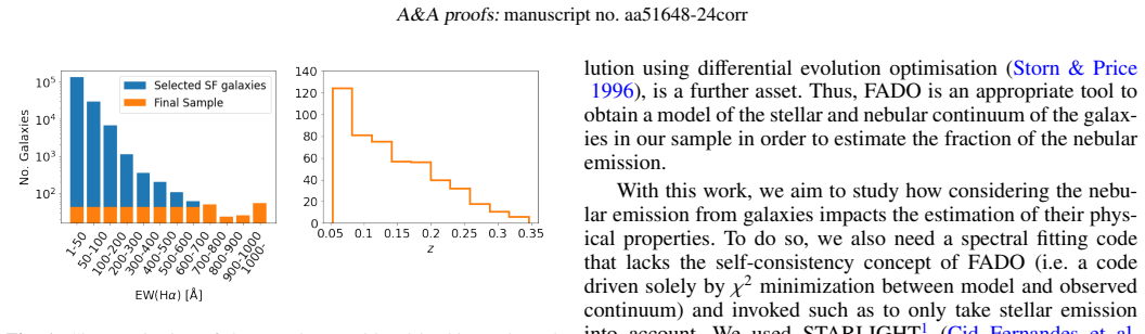
Summary. The paper seeks to establish a quantitative threshold for when neglecting the nebular continuum in optical spectral fitting leads to significant biases in derived galaxy properties. Using 500 star-forming SDSS-DR7 galaxies deliberately spread across more than two decades in EW(Halpha), the authors fit each spectrum with FADO (full-consistency stellar+nebular modelling) and STARLIGHT (stellar-only), and additionally run FADO in pure-stellar mode as a control. They find that the rest-frame EW(Halpha) and EW(Hbeta) are tight tracers of the median optical nebular contribution X_neb, and claim that for X_neb of about 8% (EW(Halpha) about 500 A, or about 375 A in a pseudo-continuum convention) the neglect of nebular emission becomes significant. Above this threshold, STARLIGHT overestimates stellar masses by 0.6 dex on average and up to 2 dex in the most extreme cases, with additional effects on age and metallicity. The paper then extrapolates the threshold to high redshift, arguing that galaxies with M* = 10^7-10^11 Msun cross it on average at z about 2-6.
Significance. If the threshold result holds, it provides a practical, citable benchmark for observers and modellers: a rest-frame EW(Halpha) cut that separates regimes where nebular continuum modelling is or is not required. This is especially timely for JWST and upcoming MOONS spectroscopy of high-redshift star-forming galaxies. The study has genuine methodological strengths: both codes are applied with the same spectral basis and extinction law, a second SSP library is used as a robustness check, and the FADO pure-stellar-mode comparison (Fig. 11) helps separate the effect of including nebular emission from code-specific fitting differences. The tracer relations in Eqs. (1)-(5) are simple and usable. The main weaknesses are statistical: the headline threshold is tied to manually chosen bin edges rather than a formal breakpoint, the paper's own 'significant difference' criterion is applied inconsistently, and the absolute X_neb scale is calibrated entirely on FADO's nebular prescription without external validation. These issues are addressable in revision, and I do not see grounds for rejection.
major comments (5)
- [Section 5.1, Table 1] The threshold criterion is not consistently applied. Under the paper's own definition of a significant difference (difference larger than 0.2 dex in either direction), the 100<=EW(Halpha)<500 A bin already contains 55% significantly different galaxies for M_curr (21% FD, 34% ST) and 57% for M_ever (22% FD, 35% ST). Thus, a statistically significant difference between the two codes is identifiable well below EW(Halpha)=500 A; what actually changes at 500 A is that the differences become one-sided, with STARLIGHT overestimating mass for more than 70% of galaxies. The statement that 'we can identify the value EW(Halpha)=500 A as the threshold for which a statistically significant difference between the two codes is identifiable' conflates the presence of significant differences with a directional bias. A formal change-point or sliding-window analysis of the continuous FADO-STARLIGHT difference as a function of EW(Halpha), with an uncertainty on the breakpoint, is needed to support the threshold claim.
- [Section 5.1, Figs. 7-10; Eq. (1)] The 500 A value is not fitted; it is one of the manually chosen bin edges (100, 500, 1000 A), and no uncertainty is quoted for the threshold or for its X_neb equivalent. Because Eq. (1) is steep in log-log space, the mapping to X_neb about 8% inherits a nontrivial uncertainty, and based on Table 1 the transition could plausibly lie anywhere within the 100-500 A interval. Please derive the threshold and its confidence interval from the continuous relation between the FADO-STARLIGHT difference and EW(Halpha) or X_neb, and quote the corresponding uncertainty on X_neb.
- [Section 3 and Section 6.1] The absolute calibration of X_neb, and therefore Eq. (1), the 8% threshold, and the 0.6-2 dex mass-bias estimates, rests entirely on FADO's nebular continuum prescription (Krueger et al. 1995; two-photon, free-free, and free-bound emission). The pure-stellar-mode control in Fig. 11 is a good check that including a nebular component matters, but it cannot detect a systematic error in FADO's nebular model itself because both modes share the same prescription. If FADO systematically over- or under-predicts the nebular continuum for a given stellar population, the reported X_neb scale and threshold would shift. This is a correctness-risk concern rather than a claim of internal circularity: the internal comparison is valid, but the absolute scale is model-dependent. I recommend validating X_neb against an independent photoionisation calculation (e.g., Cloudy run with the same ionising SEDs) or against direct nebular-continuum measurements, and at minimum stating this limitation explicitly and assessing how plausible variations in the nebular prescription would move the threshold.
- [Section 6.1, Table 1, and Fig. 9] The paper's own significance criterion does not support the claim that neglecting nebular emission significantly affects stellar metallicity. For light- and mass-weighted metallicity, the mean FADO-STARLIGHT differences are 0.03 and 0.003 dex, and even in the EW(Halpha)>=1000 A bin the light-weighted mean difference reaches only 0.09 dex. The fractions of galaxies with significant differences in the highest bins never exceed 51% for Z_L and 49% for Z_M, and the distributions retain a strong peak near zero. The abstract's statement that stellar mass, age, and metallicity are all significantly impacted is therefore an overclaim. The age-metallicity degeneracy argument in Sect. 6.1 is an inference rather than a direct measurement; please either soften the conclusions or provide direct evidence that the fitted stellar populations change above the threshold in a way that propagates systematically to the metallicity estimates.
- [Section 6.1 and Section 3] The conversion of the threshold to a pseudo-continuum EW appears arithmetically inconsistent. The text states that FADO's EW estimates are on average 0.1 dex (about 25%) higher than pseudo-continuum-based estimates. Starting from 500 A, dividing by 10^0.1 = 1.26 gives about 397 A, whereas applying a 25% reduction directly gives 375 A; the paper quotes 375 A. Please clarify which operation is intended and re-derive the scaled thresholds for Hbeta, [OIII] lambda5007, and HeI lambda5876 quoted in the summary, since these values will be used by observers who adopt pseudo-continuum conventions.
minor comments (4)
- [Abstract and Section 1] There is a grammatical issue in the abstract ('it has not been established a clear threshold'), and the text contains the typo 'redshfit' in Section 1 and again in Section 6.2.
- [Equations (1)-(5) and Section 6.1] The quoted thresholds in terms of EW(Hbeta), sSFR, EW([OIII] lambda5007), and EW(HeI lambda5876) are derived by plugging X_neb=8% into the fitted relations, but no uncertainties are propagated from the fit parameters. Please provide confidence intervals for these derived threshold values.
- [Section 6.2, Fig. 12] The construction of Fig. 12 is described only verbally: the Faisst et al. (2016) redshift evolution is normalized using mean EW(Halpha) values from Cardoso et al. (2022) in stellar-mass bins. Please specify the bin definitions, the number of galaxies per bin, and how the scatter in the EW(Halpha)-redshift relation is treated, so the claimed z about 2-6 crossing can be assessed quantitatively.
- [Section 3] The choice of 0.2 dex as the 'significant difference' threshold is reasonable and well referenced, but it is introduced after the analysis rather than as a pre-registered criterion; a sentence noting that the qualitative conclusions are not sensitive to using 0.15 or 0.25 dex would strengthen the presentation.
Circularity Check
No significant circularity: the EW(Hα)≈500 Å threshold rests on an independent FADO-vs-STARLIGHT comparison, and the X_neb≈8% value is an empirical calibration rather than a fitted prediction.
full rationale
The central claim is established by comparing FADO full-consistency fits with STARLIGHT pure-stellar fits on SDSS-DR7 galaxies, binned by EW(Hα): the paper states in Sect. 5.1 that 'we can identify the value EW(Hα)=500 Å as the threshold for which a statistically significant difference between the two codes is identifiable.' This threshold is an observed bin-edge effect in a two-code comparison, not a parameter fitted to produce the conclusion. The subsequent conversion to X_neb≈8% uses Eq. 1, a linear fit between FADO's X_neb and FADO's EW(Hα) presented in Sect. 4.1; this is an empirical calibration between two outputs of the same code rather than a prediction of a fitted input, so it does not reduce the claim to its inputs by construction. The FADO pure-stellar-mode control (Sect. 6.1) tests the effect of adding the nebular component within the same fitting machinery and supports the attribution of the FADO/STARLIGHT differences to nebular emission. Reliance on FADO's nebular prescriptions (Krüger et al. 1995) is an external physical input, and any bias there would be a correctness risk, not circularity. The paper contains heavy self-citation to FADO's development and prior FADO applications, but these are normal tool citations and are not load-bearing in the sense of a uniqueness theorem or an unverified ansatz. The paper also explicitly acknowledges that sub-threshold effects may exist ('we note that it is possible that galaxies with median nebular contributions lower than 8% are impacted'), further indicating that the threshold is a data-driven observation rather than a forced identity. Overall, no step in the derivation chain is equivalent to its inputs by definition.
Assumptions & free parameters
free parameters (11)
- log X_neb vs log EW(Hα) slope =
0.98 ± 0.05
- log X_neb vs log EW(Hα) intercept =
-1.77 ± 0.13
- log X_neb vs log EW(Hβ) slope =
1.03 ± 0.03
- log X_neb vs log EW(Hβ) intercept =
-1.19 ± 0.05
- log X_neb vs log sSFR slope =
0.50 ± 0.03
- log X_neb vs log sSFR intercept =
4.80 ± 0.24
- Quadratic coefficients for [OIII] relation =
0.08, 0.23, -0.24
- log X_neb vs log EW(HeI5876) slope =
0.96 ± 0.02
- log X_neb vs log EW(HeI5876) intercept =
-0.20 ± 0.03
- Significant difference threshold =
0.2 dex
- FADO-to-pseudo-continuum EW scaling =
0.1 dex (~25%)
assumptions (5)
- domain assumption The BPT diagram classification correctly identifies star-forming galaxies whose ionizing radiation is not dominated by AGN.
- domain assumption FADO's photoionisation prescription (Krueger et al. 1995; two-photon, free-free, free-bound) accurately models the nebular continuum.
- ad hoc to paper The 0.2 dex typical accuracy of FADO and STARLIGHT is a valid threshold for significant difference in derived galaxy properties.
- domain assumption The Faisst et al. (2016) empirical EW(Hα) redshift evolution, with slopes 1.8 for z<2 and 1.3 for 2≤z<6, applies to galaxies across stellar mass and can be normalized with local FADO/Cardoso data.
- ad hoc to paper The median nebular contribution X_neb over the 3000-9000 Å window is a representative measure of the nebular impact on spectral fits.
Cite this review
Pith. "Pith review of Importance of modelling the nebular continuum in galaxy spectra." pith.science (2026). https://pith.science/paper/BEX2PCI2
@misc{pith2026241212060,
  author       = {Pith},
  title        = {Pith review of: Importance of modelling the nebular continuum in galaxy spectra},
  year         = {2026},
  howpublished = {\url{https://pith.science/paper/BEX2PCI2}},
  note         = {Machine review of arXiv:2412.12060}
}
abstract
The neglect of modelling both stellar and nebular emission significantly affects the derived physical properties of galaxies, particularly those with high star formation rates. While this issue has been studied, it has not been established a clear threshold for a significant impact on the estimated physical properties of galaxies due to accounting for both stellar and nebular emission. We analyse galaxies from SDSS-DR7 across a wide range of star-forming activity levels, comparing the results obtained from two spectral fitting tools: FADO (which considers both stellar and nebular continuum) and STARLIGHT (only considers the stellar continuum). A strong linear correlation is found between the rest-frame H$\alpha$ and H$\beta$ equivalent widths (EWs) and the optical nebular contribution, identifying these as reliable tracers. The results show that when the nebular contribution exceeds 8% (corresponding to EW(H$\alpha$)$\simeq$500 \r{A} and EW(H$\beta$)$\simeq$110 \r{A}), there is a significant impact on the estimation of galaxy properties, namely stellar mass, age and metallicity. Our results highlight the importance of taking into account both the stellar and nebular continuum when analysing the optical spectra of star-forming galaxies. In particular, this is a fundamental aspect for galaxies with a rest-frame EW(H$\alpha$)$\gtrsim$500 \r{A} (or the scaled value of 375 \r{A} for pseudo-continuum measures). At low redshifts, this mostly impacts extreme emission line galaxies, while at higher redshifts it becomes a dominant aspect given the higher star-forming activity in the younger Universe. In light of current JWST observations and future instruments designed for high-redshift observations, such as MOONS, this reveals as a critical issue to take into consideration.
Figures


Figures from the paper (7 more)


Reference graph
Works this paper leans on
-
[1]
N., Adelman-McCarthy, J
Abazajian, K. N., Adelman-McCarthy, J. K., Ag \"u eros, M. A., et al.\ 2009, , 182, 543
2009
-
[2]
Alongi, M., Bertelli, G., Bressan, A., et al.\ 1993, , 97, 851
1993
-
[3]
O., P \'e rez-Montero, E., & V \' lchez, J
Amor \' n, R. O., P \'e rez-Montero, E., & V \' lchez, J. M.\ 2010, , 715, L128
2010
-
[4]
Amor \' n, R., P \'e rez-Montero, E., Contini, T., et al.\ 2015, , 578, A105
2015
-
[5]
& Fritze-v
Anders, P. & Fritze-v. Alvensleben, U.\ 2003, , 401, 1063
2003
-
[6]
Atek, H., Siana, B., Scarlata, C., et al.\ 2011, , 743, 121
2011
-
[7]
A., Phillips, M
Baldwin, J. A., Phillips, M. M., & Terlevich, R.\ 1981, , 93, 5
1981
-
[8]
M., Papaderos, P., et al.\ 2022, , 663, A29
Breda, I., Vilchez, J. M., Papaderos, P., et al.\ 2022, , 663, A29
2022
Show all 103 references
-
[9]
Bressan, A., Fagotto, F., Bertelli, G., et al.\ 1993, , 100, 647
1993
-
[10]
Brinchmann, J., Charlot, S., White, S. D. M., et al.\ 2004, , 351, 1151
2004
-
[11]
W., Salzer, J
Brunker, S. W., Salzer, J. J., Janowiecki, S., et al.\ 2020, , 898, 68
2020
-
[12]
& Charlot, S.\ 2003, , 344, 1000
Bruzual, G. & Charlot, S.\ 2003, , 344, 1000
2003
-
[13]
Boyett, K. N. K., Stark, D. P., Bunker, A. J., et al.\ 2022, , 513, 4451
2022
-
[14]
J., Curtis-Lake, E., et al.\ 2024, , 535, 1796
Boyett, K., Bunker, A. J., Curtis-Lake, E., et al.\ 2024, , 535, 1796
2024
-
[15]
J., NIRSPEC Instrument Science Team, & JADESs Collaboration\ 2020, Uncovering Early Galaxy Evolution in the ALMA and JWST Era, IAU Proc., 352, 342
Bunker, A. J., NIRSPEC Instrument Science Team, & JADESs Collaboration\ 2020, Uncovering Early Galaxy Evolution in the ALMA and JWST Era, IAU Proc., 352, 342
2020
-
[16]
C., et al.\ 2000, , 533, 682
Calzetti, D., Armus, L., Bohlin, R. C., et al.\ 2000, , 533, 682
2000
-
[17]
J., Katz, H., Witten, C., et al.\ 2024, , 534, 523
Cameron, A. J., Katz, H., Witten, C., et al.\ 2024, , 534, 523
2024
-
[18]
I., Rinaldi, P., Iani, E., et al.\ 2024, , 969, 159
Caputi, K. I., Rinaldi, P., Iani, E., et al.\ 2024, , 969, 159
2024
-
[19]
Cardamone, C., Schawinski, K., Sarzi, M., et al.\ 2009, , 399, 1191
2009
-
[20]
A., Clayton, G
Cardelli, J. A., Clayton, G. C., & Mathis, J. S.\ 1989, , 345, 245
1989
-
[21]
Cardoso, L. S. M., Gomes, J.-M., & Papaderos, P.\ 2016, , 594, L2
2016
-
[22]
Cardoso, L. S. M., Gomes, J. M., & Papaderos, P.\ 2019, , 622, A56
2019
-
[23]
Cardoso, L. S. M., Gomes, J. M., Papaderos, P., et al.\ 2022, , 667, A11
2022
-
[24]
C., McLure, R
Carnall, A. C., McLure, R. J., Dunlop, J. S., et al.\ 2018, , 480, 4379
2018
-
[25]
Chabrier, G.\ 2003, Apj, 586, L133
2003
-
[26]
Cid Fernandes, R., Mateus, A., Sodr \'e , L., et al.\ 2005, , 358, 363
2005
-
[27]
Cid Fernandes, R., Stasi \'n ska, G., Mateus, A., et al.\ 2011, , 413, 1687
2011
-
[28]
M., Garc \' a Benito, R., et al.\ 2014, , 561, A130
Cid Fernandes, R., Gonz \'a lez Delgado, R. M., Garc \' a Benito, R., et al.\ 2014, , 561, A130
2014
-
[29]
& MOONS Consortium\ 2016, Multi-Object Spectroscopy in the Next Decade: Big Questions, Large Surveys, and Wide Fields, 507, 109
Cirasuolo, M. & MOONS Consortium\ 2016, Multi-Object Spectroscopy in the Next Decade: Big Questions, Large Surveys, and Wide Fields, 507, 109
2016
-
[30]
Cirasuolo, M., Fairley, A., Rees, P., et al.\ 2020, The Messenger, 180, 10
2020
-
[31]
Conroy, C.\ 2013, , 51, 393
2013
-
[32]
R., Vacca, W
Corbin, M. R., Vacca, W. D., Cid Fernandes, R., et al.\ 2006, , 651, 861
2006
-
[33]
R., Simons, R
Davis, K., Trump, J. R., Simons, R. C., et al.\ 2024, , 974, 42
2024
-
[34]
J., Willott, C., Alberts, S., et al.\ 2023, arXiv e-prints [ [arXiv] 2306.02465 ]
Eisenstein, D. J., Willott, C., Alberts, S., et al.\ 2023, arXiv e-prints [ [arXiv] 2306.02465 ]
2023 arXiv
-
[35]
P., Chevallard, J., et al.\ 2021, , 500, 5229
Endsley, R., Stark, D. P., Chevallard, J., et al.\ 2021, , 500, 5229
2021
-
[36]
P., Whitler, L., et al.\ 2023, , 524, 2312
Endsley, R., Stark, D. P., Whitler, L., et al.\ 2023, , 524, 2312
2023
-
[37]
Fagotto, F., Bressan, A., Bertelli, G., et al.\ 1994a, , 104, 365
-
[38]
Fagotto, F., Bressan, A., Bertelli, G., et al.\ 1994b, , 105, 29
-
[39]
L., Capak, P., Hsieh, B
Faisst, A. L., Capak, P., Hsieh, B. C., et al.\ 2016, , 821, 122
2016
-
[40]
L., Bagley, M
Finkelstein, S. L., Bagley, M. B., Ferguson, H. C., et al.\ 2023, , 946, L13
2023
-
[41]
L., Leung, G
Finkelstein, S. L., Leung, G. C. K., Bagley, M. B., et al.\ 2024, , 969, L2
2024
-
[42]
G., Franx, M., et al.\ 2012, , 757, L22
Fumagalli, M., Patel, S. G., Franx, M., et al.\ 2012, , 757, L22
2012
-
[43]
Girardi, L., Bressan, A., Chiosi, C., et al.\ 1996, , 117, 113
1996
-
[44]
Gomes, J. M. & Papaderos, P.\ 2017, , 603, A63
2017
-
[45]
Gunawardhana, M. L. P., Brinchmann, J., Weilbacher, P. M., et al.\ 2020, , 497, 3860
2020
-
[46]
C., et al.\ 2024, , 528, 6593
Guo, Y., Sengupta, C., Scott, T. C., et al.\ 2024, , 528, 6593
2024
-
[47]
G., Izotov, Y
Guseva, N. G., Izotov, Y. I., Papaderos, P., et al.\ 2001, , 378, 756
2001
-
[48]
G., Izotov, Y
Guseva, N. G., Izotov, Y. I., Papaderos, P., et al.\ 2007, , 464, 885
2007
-
[49]
I., et al.\ 2024, , submitted, [ [arXiv] 2406.18207 ]
Iani, E., Rinaldi, P., Caputi, K. I., et al.\ 2024, , submitted, [ [arXiv] 2406.18207 ]
2024 arXiv
-
[50]
I., Lipovetsky, V
Izotov, Y. I., Lipovetsky, V. A., Chaffee, F. H., et al.\ 1997, , 476, 698
1997
-
[51]
I., Guseva, N
Izotov, Y. I., Guseva, N. G., & Thuan, T. X.\ 2011, , 728, 161
2011
-
[52]
D., Leja, J., Conroy, C., et al.\ 2021, , 254, 22
Johnson, B. D., Leja, J., Conroy, C., et al.\ 2021, , 254, 22
2021
-
[53]
C.\ 1998, , 36, 189
Kennicutt, R. C.\ 1998, , 36, 189
1998
-
[54]
Alvensleben, U., & Loose, H.-H.\ 1995, , 303, 41
Krueger, H., Fritze-v. Alvensleben, U., & Loose, H.-H.\ 1995, , 303, 41
1995
-
[55]
Labb \'e , I., van Dokkum, P., Nelson, E., et al.\ 2023, , 616, 266
2023
-
[56]
Lagos, P., Telles, E., Nigoche-Netro, A., et al.\ 2011, , 142, 162
2011
-
[57]
I., Scott, T
Lagos, P., Loubser, S. I., Scott, T. C., et al.\ 2022, , 516, 5487
2022
-
[58]
L., Hutchison, T
Larson, R. L., Hutchison, T. A., Bagley, M., et al.\ 2023, , 958, 141
2023
-
[59]
D., et al.\ 1999, , 123, 3
Leitherer, C., Schaerer, D., Goldader, J. D., et al.\ 1999, , 123, 3
1999
-
[60]
D., Conroy, C., et al.\ 2017, , 837, 170
Leja, J., Johnson, B. D., Conroy, C., et al.\ 2017, , 837, 170
2017
-
[61]
D., et al.\ 2024, , 969, L5
Li, Y., Leja, J., Johnson, B. D., et al.\ 2024, , 969, L5
2024
-
[62]
Llerena, M., Amor \' n, R., Pentericci, L., et al.\ 2024, , 691, A59
2024
-
[63]
& Dickinson, M.\ 2014, , 52, 415
Madau, P. & Dickinson, M.\ 2014, , 52, 415
2014
-
[64]
Maiolino, R., Cirasuolo, M., Afonso, J., et al.\ 2020, The Messenger, 180, 24
2020
-
[65]
Mannucci, F., Cresci, G., Maiolino, R., et al.\ 2010, , 408, 2115
2010
-
[66]
J., Cullen, F., et al.\ 2016, , 460, 3587
M \'a rmol-Queralt \'o , E., McLure, R. J., Cullen, F., et al.\ 2016, , 460, 3587
2016
-
[67]
P., Brammer, G., et al.\ 2024, , 963, 129
Matthee, J., Naidu, R. P., Brammer, G., et al.\ 2024, , 963, 129
2024
-
[68]
M., et al.\ 2023, , 946, L39
McKinney, J., Finnerty, L., Casey, C. M., et al.\ 2023, , 946, L39
2023
-
[69]
Miranda, H., Pappalardo, C., Papaderos, P., et al.\ 2023, , 669, A16
2023
-
[70]
Nakajima, K., Ouchi, M., Xu, Y., et al.\ 2022, , 262, 3
2022
-
[71]
I., Fricke, K
Papaderos, P., Izotov, Y. I., Fricke, K. J., et al.\ 1998, , 338, 43
1998
-
[72]
I., Thuan, T
Papaderos, P., Izotov, Y. I., Thuan, T. X., et al.\ 2002, , 393, 461
2002
-
[73]
& \"O stlin, G.\ 2012, , 537, A126
Papaderos, P. & \"O stlin, G.\ 2012, , 537, A126
2012
-
[74]
Papaderos, P., Breda, I., Humphrey, A., et al.\ 2022, , 658, A74
2022
-
[75]
Papaderos, P., \"O stlin, G., & Breda, I.\ 2023, , 673, A30
2023
-
[76]
Pappalardo, C., Cardoso, L. S. M., Michel Gomes, J., et al.\ 2021, , 651, A99
2021
-
[77]
G., Barro, G., Rieke, G
P \'e rez-Gonz \'a lez, P. G., Barro, G., Rieke, G. H., et al.\ 2024, , 968, 4
2024
-
[78]
Popesso, P., Concas, A., Cresci, G., et al.\ 2023, , 519, 1526
2023
-
[79]
A., Shapley, A
Reddy, N. A., Shapley, A. E., Sanders, R. L., et al.\ 2018, , 869, 92
2018
-
[80]
E., Nidever, D
Reines, A. E., Nidever, D. L., Whelan, D. G., et al.\ 2010, , 708, 26
2010
-
[81]
Rieke, M.\ 2020, Uncovering Early Galaxy Evolution in the ALMA and JWST Era, 352, 337
2020
-
[82]
G., Riffel, R
Riffel, R., Dahmer-Hahn, L. G., Riffel, R. A., et al.\ 2022, , 512, 3906
2022
-
[83]
Roberts-Borsani, G., Treu, T., Shapley, A., et al.\ 2024, , 976, 193
2024
-
[84]
J., MacAlpine, G
Salzer, J. J., MacAlpine, G. M., & Boroson, T. A.\ 1989, , 70, 479
1989
-
[85]
J., Jones, G
Saxena, A., Bunker, A. J., Jones, G. C., et al.\ 2024, , 684, A84
2024
-
[86]
& de Barros, S.\ 2009, , 502, 423
Schaerer, D. & de Barros, S.\ 2009, , 502, 423
2009
-
[87]
& de Barros, S.\ 2010, , 515, A73
Schaerer, D. & de Barros, S.\ 2010, , 515, A73
2010
-
[88]
Schlafly, E. F. & Finkbeiner, D. P.\ 2011, , 737, 103
2011
-
[89]
J., Finkbeiner, D
Schlegel, D. J., Finkbeiner, D. P., & Davis, M.\ 1998, , 500, 525
1998
-
[90]
Alvensleben, U., M \"o ller, C
Schulz, J., Fritze-v. Alvensleben, U., M \"o ller, C. S., et al.\ 2002, , 392, 1
2002
-
[91]
Simmonds, C., Tacchella, S., Maseda, M., et al.\ 2023, , 523, 5468
2023
-
[92]
J., Franx, M., et al.\ 2015, , 801, 122
Smit, R., Bouwens, R. J., Franx, M., et al.\ 2015, , 801, 122
2015
-
[93]
S., Steinhardt, C
Speagle, J. S., Steinhardt, C. L., Capak, P. L., et al.\ 2014, , 214, 15
2014
-
[94]
on Evolutionary Computation,842, 844
Storn, R., & Price, K.V., 1996, Minimizing the real function of the ICEC’96contest by differential evolution, IEEE conf. on Evolutionary Computation,842, 844
1996
-
[95]
Sun, F., Egami, E., Pirzkal, N., et al.\ 2023, , 953, 53
2023
-
[96]
Terlevich, R., Melnick, J., Masegosa, J., et al.\ 1991, , 91, 285
1991
-
[97]
Wang, B., Leja, J., Atek, H., et al.\ 2024, , 963, 74
2024
-
[98]
Weilbacher, P. M. & Fritze-v. Alvensleben, U.\ 2001, , 373, L9
2001
-
[99]
M., Lovell, C
Wilkins, S. M., Lovell, C. C., & Stanway, E. R.\ 2019, , 490, 5359
2019
-
[100]
N., Rix, H.-W., et al.\ 2011, , 742, 111
van der Wel, A., Straughn, A. N., Rix, H.-W., et al.\ 2011, , 742, 111
2011
-
[101]
G., Adelman, J., Anderson, J
York, D. G., Adelman, J., Anderson, J. E., et al.\ 2000, , 120, 1579
2000
-
[102]
, " * write output.state after.block = add.period write newline
ENTRY address archiveprefix author booktitle chapter edition editor howpublished institution eprint journal key month note number organization pages publisher school series title type volume year label extra.label sort.label short.list INTEGERS output.state before.all mid.sent...
-
[103]
write newline
" write newline "" before.all 'output.state := FUNCTION n.dashify 't := "" t empty not t #1 #1 substring "-" = t #1 #2 substring "--" = not "--" * t #2 global.max substring 't := t #1 #1 substring "-" = "-" * t #2 global.max substring 't := while if t #1 #1 substring * t #2 gl...
Reviewed August 11, 2026 · model on record in the stance chip above.
Discussion (0). Continue with ORCID to comment.