REVIEW 3 major objections 5 minor 1 cited by
Cosmic Multipoles in Galaxy Surveys Part I: How Inferences Depend on Source Counts and Masks
T0 review · 3 major / 5 minor · reviewed 2026-08-11 · deepseek-v4-flash
Pith's one-line read A Bayesian fit of traceless-symmetric-tensor multipole templates recovers dipole, quadrupole, and octupole parameters from galaxy count maps even when half the sky is masked, with no mode coupling between harmonics.
desk verdict Useful survey-planning numbers from a sound in-sample Bayesian pipeline, but the no-mode-coupling claim is conditional on model completeness. read the letter →
The pith
A machine-rendered reading of the paper's core claim, the machinery that carries it, and where it could break.
The reading
What carries the argument
The central object is the traceless symmetric tensor multipole: for order $\ell$, take the outer product of $\ell$ unit vectors, symmetrize over all index permutations, and subtract the traces, leaving a tensor whose full contraction with a pixel's unit direction vector gives the signal at that pixel, scaled by an amplitude ($D$, $Q$, or $\mathcal{O}$). Expected cell counts are the monopole density times (1 + signal), and observed counts are Poisson draws at that rate. Bayesian inference over the amplitudes and unit-vector directions, with nested sampling for the marginal likelihood, yields posterior distributions and log Bayes factors comparing monopole, dipole, dipole+quadrupole, and dipole+octupole models, and the Kullback-Leibler divergence between posterior and prior measures how much information the data carries. Because the templates are fitted directly rather than projected onto a complete-sky harmonic basis, the orthogonality failure that produces mode mixing on masked skies never enters the calculation.
What would settle it
Take the paper's pipeline and apply it to a real catalogue with known systematics, such as CatWISE2020: subtract the best-fit monopole+dipole+quadrupole template and compute the angular power spectrum of the residuals. Significant residual power at $\ell \geq 4$, or a dipole amplitude that shifts outside its credible interval when an octupole is added to the fit, would show that unmodeled angular structure does leak into the inferred dipole on real skies. A purely synthetic version of the same test is to inject an unmodeled higher-order or axis-mismatched multipole into the Poisson samples and check whether the dipole posterior moves.
Extended reading notes
Core claim
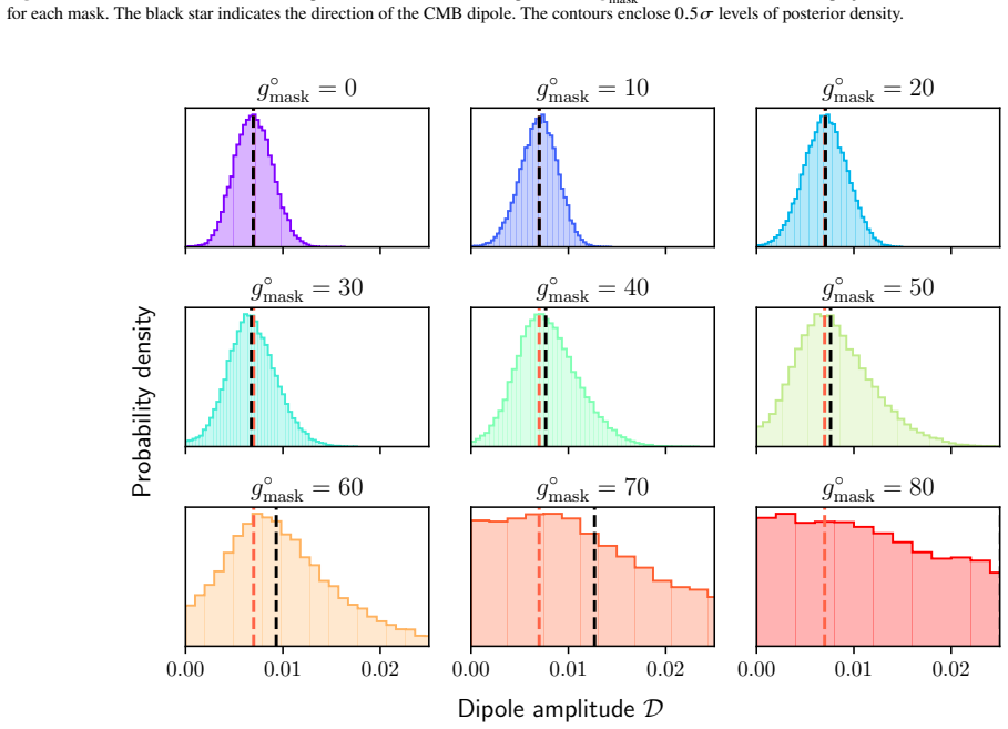
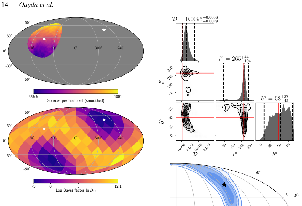
On its own terms, the paper's central discovery is that multipole inference on the celestial sphere does not need the full-sky orthonormality of spherical harmonics. Each multipole is constructed as a traceless symmetric tensor built from unit vectors — the dipole as $d_j\hat{p}_j$, the quadrupole as $Q_{jk}\hat{p}_j\hat{p}_k$, the octupole as $O_{jkl}\hat{p}_j\hat{p}_k\hat{p}_l$ — and these templates are fitted to Poisson-sampled pixel counts through a Bayesian likelihood, with nested sampling supplying the evidence for model comparison. For samples with a Galactic-plane mask leaving $f_{\rm sky}=0.5$, the paper reports that the injected dipole, quadrupole, and octupole parameters are recovered accurately, with no mode coupling between $\ell=1$, $\ell=2$, and $\ell=3$; even discontinuous masks resembling the 391 pointings of a real telescope survey pose no added difficulty. It further establishes that the information content of a survey is set mainly by total source count and the angular radius of visible sky, that a dipole of the CMB-implied amplitude $D=0.007$ needs about $N\approx5\times10^5$ sources for strong model support, and that small patches placed near the dipole equator can deliver a $\geq4\sigma$ exclusion of a $2\times$ CMB-amplitude dipole.
Load-bearing premise
The load-bearing premise is that a real galaxy count map is essentially a Poisson realization of a smooth low-order multipole model, with no angular structure beyond the dipole, quadrupole, and octupole being fitted; if a real catalogue carries extra structure (ecliptic-plane systematics, source clustering, multi-component radio sources), the claimed absence of cross-talk between fitted modes is not guaranteed.
Editorial extensions
If this is right
- The CatWISE2020 dipole measurement that triggered the tension can be revisited: fitting a simultaneous dipole+quadrupole model separates the kinematic dipole from the strong ecliptic-bias quadrupole instead of letting higher-order power leak into the $\ell=1$ estimate.
- Small-footprint surveys are viable: a 40-degree-radius slice needs about 42 million sources and an 80-degree slice about 6.6 million sources to reach the paper's $D_{\rm KL}=5.5$ threshold, at which the dipole is constrained to $\geq4\sigma$ significance against a $2\times$ CMB-amplitude dipole.
- There is a practical detection floor: near $N\approx5\times10^5$ sources, the Bayes factor for a dipole over a monopole crosses 'overwhelming' support at the CMB-implied amplitude, so smaller samples cannot claim either a detection or a null result for the cosmic dipole.
- Discontinuous surveys are not handicapped: a scattered mask built from 391 individual pointings of the MALS telescope recovers the dipole with the same KL divergence as a continuous slice of equal angular breadth, and the paper estimates $N\approx1.2$ million sources in that geometry would suffice for a roughly $3\sigma$ discrimination of a $2\times$ CMB dipole from the CMB expectation.
- The framework generalizes to arbitrary multipole order, so future wide surveys such as SKA, Euclid, and LSST can be analyzed with a unified low-order multipole model rather than a truncated spherical-harmonic expansion.
Reading between the lines
- Extension the paper leaves implicit: its no-crosstalk claim is demonstrated only for skies that are exactly Poisson realizations of the fitted low-order models; injecting an unmodeled mode (a higher $\ell$, or a quadrupole whose axis is not in the fitted set) into the same pipeline is a direct test of whether unmodeled real-world structure — such as CatWISE2020's ecliptic systematics — would reint
- The prior-sensitivity analysis implies that part of the scatter across published dipole amplitudes may come from estimator choice: a flat-Cartesian-component prior, which the paper shows biases amplitudes upward, is effectively what least-squares template fits impose (the paper tests such a fit on a pure monopole sample and recovers a spurious $D\approx0.0035$), pushing low-information samples tow
- The near-linear growth of per-source information with slice radius suggests a design rule for future surveys: for a fixed source budget, angular breadth buys more dipole constraining power than depth, so wide shallow coverage should outperform deep narrow pointing for cosmic-dipole science.
- Because the iso-information contours (e.g., $D_{\rm KL}=5.5$) are calibrated against the paper's specific priors and amplitudes, the quoted source-count requirements should be re-derived, not reused, when an analysis adopts different priors or targets different dipole amplitudes.
Editorial analysis
A structured set of objections, weighed in public.
Referee Report
Summary. The paper develops a Bayesian method for fitting source-count multipoles (dipole, quadrupole, octupole) using traceless symmetric tensor templates evaluated directly on pixel counts, rather than spherical harmonic decomposition. The authors generate synthetic Poisson catalogues with injected multipole signals, apply Galactic-plane masks of varying severity and a range of source counts, and use nested sampling to recover amplitudes and directions, with Bayes factors for model comparison. They report that the method recovers injected parameters even at f_sky = 0.5, concluding that mode coupling on masked skies is not a concern for their approach. They also derive source-count thresholds for dipole inference on small and discontinuous footprints and demonstrate sensitivity to prior choice. The paper is structured as a simulation study with propositions summarizing the main findings.
Significance. If the central no-crosstalk claim holds, the method offers a principled way to separate a cosmological dipole from higher-order angular structure in masked galaxy surveys, directly relevant to the current dipole-tension debate. The quantitative source-count thresholds (e.g., N ≈ 500,000 for strong support at D = 0.007) and the KL-divergence-based survey-design framework are useful, concrete deliverables for planning future dipole measurements. The paper is also commendable for explicitly demonstrating prior sensitivity and for using a proper Poisson likelihood, even though the constant terms are omitted. The main limitation is that the key robustness claim is demonstrated only for signals drawn from the same parametric family that is fitted, so the significance for real catalogues is conditional on model completeness; the paper acknowledges this in places but does not test it.
major comments (3)
- [Section 5.1, Proposition 4; Abstract] The claim that 'mode coupling on masked skies is not a concern for our approach' is established only for Poisson realizations of the fitted model family. The paper itself notes in the §3.2.1 footnote that independent source positions are broken for multi-component radio sources, and in §2 it describes CatWISE2020 as having an ecliptic bias and higher-order residuals. Because the traceless tensor templates are orthogonal only over the full sphere, unmodeled angular structure (e.g., an ℓ ≥ 4 component or a smooth declination-dependent systematic) can project onto the ℓ = 1 template over the unmasked region and bias the inferred dipole. The current experiments do not include such unmodeled modes, so Proposition 4 overstates the robustness. Please either add simulations with unmodeled angular structure and demonstrate that the dipole is still unbiased, or reformulate Proposition 4 as valid within the assumed model family.
- [Section 4.4] The octupole crosstalk test consists of a single UltraNest run with N ≈ 98 million and f_sky = 0.5, and Proposition 4's 'combinations of these underlying multipole signals' is never tested with dipole, quadrupole, and octupole present simultaneously. A single high-source-count run is weak evidence for the general no-crosstalk claim, especially because the proposed application to real catalogues involves much lower source counts. Additional verification with repeated runs at survey-relevant source counts, and with simultaneous dipole+quadrupole+octupole injection, is needed to support the proposition as stated.
- [Section 3.3.1, priors] The direction prior is written as 'θ ∼ cos−1(1−2u) for u ∼ U(0, 0.1)'. As written, u ∈ [0, 0.1] restricts θ to [0, arccos(0.8)] ≈ [0°, 36.9°], which is not uniform over the sphere and would bias every direction inference. The stated goal of uniform coverage over the sphere requires u ∼ U(0, 1). Given the sensible direction posteriors reported later, this is presumably a typographical error, but the formula must be corrected because it is load-bearing for all directional results.
minor comments (5)
- [Figure 1 caption] The caption labels the middle-right column as 'Dipole and quadrupole sample S4'; this should be Sample S3, since S4 is the dipole and octupole sample.
- [Section 3.2.2] The text states that samples are generated with values of N up to 10,000,000, but Section 4.4 uses N ≈ 98 million for Sample S4; please clarify that S4 uses a larger source-count regime.
- [Section 4.5.1] The fitted function for the KL divergence is typeset ambiguously as 'D_KL(N,r°) = A log10 N + (r°)B − N C + D'; please clarify the intended functional form and report the fitted constants.
- [Section 3.3.1] The expression 'θ ∼ cos−1(1−2u)' is missing a closing parenthesis; it should read 'cos−1(1−2u)' with the parenthesis closed after 'u'.
- [Data Availability] The data availability statement says data 'will be made available with a reasonable request' but does not mention releasing the analysis code; for a methods-oriented paper, archiving the code would substantially aid reproducibility.
Circularity Check
No significant circularity: the paper's claims are in-sample simulation validations with explicit model-completeness caveats, not reductions to their inputs.
full rationale
The paper's central claims are empirical demonstrations on synthetic catalogues, not derivations that reduce to their inputs. The data are generated from the same parametric multipole family that is later fitted (Eqs. 6, 27, 28 for generation; Eq. 30 for the Poisson likelihood), but this is standard simulation validation. Recovery under masks and Poisson noise is nontrivial: the traceless-symmetric-tensor templates are not orthogonal over a masked sky, so the posterior concentration shown in Sections 4.3 and 4.4 is a substantive result rather than a tautology. The claimed robustness is explicitly conditional: Proposition 4 refers to 'samples consisting of combinations of these underlying multipole signals', and the paper acknowledges real-catalogue complications such as multi-component radio sources (§3.2.1) and ecliptic/declination-dependent systematics with higher-order residuals (§2). The source-count thresholds are derived from their own simulations and are explicitly prior-dependent, with Section 4.6 providing a cautionary demonstration of prior sensitivity; no fitted parameter is relabelled as an external prediction. Self-citations to Mittal et al. (2024) and Oayda et al. (2024) for the statistical machinery are not load-bearing because the likelihood, priors, and models are fully written out in the text. No uniqueness theorem or ansatz is imported from the authors' prior work. The paper is therefore self-contained as a simulation study, and the stated limitations prevent the central claims from being circular.
Assumptions & free parameters
free parameters (5)
- Injected dipole amplitude D in samples S1, S3, S4 =
0.007
- Injected quadrupole amplitude Q in samples S2, S3 =
0.014
- Injected octupole amplitude O in sample S4 =
0.03
- Prior widths for amplitudes
- KL divergence interpolation constants A, B, C, D =
not reported
assumptions (4)
- domain assumption Ellis-Baldwin relation D = (2 + x(1 + alpha)) beta for the expected kinematic dipole in galaxy counts.
- domain assumption Source positions are independent Poisson draws with rate equal to the template signal.
- standard math The traceless symmetric rank-l tensor expansion is equivalent to the standard spherical harmonic multipole expansion.
- domain assumption Nested sampling estimates of the posterior and evidence are converged for the reported runs.
Cite this review
Pith. "Pith review of Cosmic Multipoles in Galaxy Surveys Part I: How Inferences Depend on Source Counts and Masks." pith.science (2026). https://pith.science/paper/ICNKTD4N
@misc{pith2026241212600,
  author       = {Pith},
  title        = {Pith review of: Cosmic Multipoles in Galaxy Surveys Part I: How Inferences Depend on Source Counts and Masks},
  year         = {2026},
  howpublished = {\url{https://pith.science/paper/ICNKTD4N}},
  note         = {Machine review of arXiv:2412.12600}
}
abstract
We present a new approach to constructing and fitting dipoles and higher-order multipoles in synthetic galaxy samples over the sky. Within our Bayesian paradigm, we illustrate that this technique is robust to masked skies, allowing us to make credible inferences about the relative contributions of each multipole. We also show that dipoles can be recovered in surveys with small footprints, determining the requisite source counts required for concrete estimation of the dipole parameters. This work is motivated by recent probes of the cosmic dipole in galaxy catalogues. Namely, the kinematic dipole of the Cosmic Microwave Background, as arising from the motion of our heliocentric frame at $\approx 370\ \text{km}\,\text{s}^{-1}$, implies that an analogous dipole should be observed in the number counts of galaxies in flux-density-limited samples. Recent studies have reported a dipole aligning with the kinematic dipole but with an anomalously large amplitude. Accordingly, our new technique will be important as forthcoming galaxy surveys are made available and for revisiting previous data.
Figures


Figures from the paper (13 more)






Forward citations
Cited by 1 Pith paper
-
The Cosmological Dipole in Tilted Anisotropic Universes
In tilted Bianchi cosmologies, a 10^-3 dipole is impossible under current shear and curvature bounds except possibly for a Khronon field.
Reference graph
Works this paper leans on
-
[1]
, " * write output.state after.block = add.period write newline
ENTRY address archivePrefix author booktitle chapter doi edition editor eprint howpublished institution journal key month note number organization pages publisher school series title type volume year label extra.label sort.label short.list INTEGERS output.state before.all mid.sentence after.sentence after.block FUNCTION init.state.consts #0 'before.all :=...
-
[2]
write newline
" write newline "" before.all 'output.state := FUNCTION format.doi doi empty "" "doi:" doi * if FUNCTION format.eprint eprint empty "" archivePrefix empty "" archivePrefix ":" * if eprint field.or.null * if FUNCTION format.pid eprint empty format.doi format.eprint if FUNCTION n.dashify 't := "" t empty not t #1 #1 substring "-" = t #1 #2 substring "--" = ...
-
[3]
Abghari A., Bunn E. F., Hergt L. T., Li B., Scott D., Sullivan R. M., Wei D., 2024, @doi [arXiv e-prints] 10.48550/arXiv.2405.09762 , https://ui.adsabs.harvard.edu/abs/2024arXiv240509762A p. arXiv:2405.09762
-
[4]
Astropy Collaboration et al., 2022, @doi [apj] 10.3847/1538-4357/ac7c74 , https://ui.adsabs.harvard.edu/abs/2022ApJ...935..167A 935, 167
-
[5]
Baleisis A., Lahav O., Loan A. J., Wall J. V., 1998, @doi [ ] 10.1046/j.1365-8711.1998.01536.x , https://ui.adsabs.harvard.edu/abs/1998MNRAS.297..545B 297, 545
arXiv 1998
-
[6]
Bengaly C. A., Maartens R., Santos M. G., 2018, @doi [ ] 10.1088/1475-7516/2018/04/031 , 2018, 031
-
[7]
Bengaly C. A. P., Siewert T. M., Schwarz D. J., Maartens R., 2019, @doi [ ] 10.1093/mnras/stz832 , https://ui.adsabs.harvard.edu/abs/2019MNRAS.486.1350B 486, 1350
-
[8]
Blake C., Wall J., 2002, @doi [ ] 10.1038/416150a , https://ui.adsabs.harvard.edu/abs/2002Natur.416..150B 416, 150
doi:10.1038/416150a 2002
Show all 68 references
-
[9]
Buchner J., 2016, @doi [Statistics and Computing] 10.1007/s11222-014-9512-y , https://ui.adsabs.harvard.edu/abs/2016S&C....26..383B 26, 383
2016 doi
-
[10]
Buchner J., 2019, @doi [ ] 10.1088/1538-3873/aae7fc , https://ui.adsabs.harvard.edu/abs/2019PASP..131j8005B 131, 108005
2019 doi
-
[11]
Buchner J., 2021, @doi [The Journal of Open Source Software] 10.21105/joss.03001 , https://ui.adsabs.harvard.edu/abs/2021JOSS....6.3001B 6, 3001
2021 doi
-
[12]
Buchner J., 2023, @doi [Statistics Surveys] 10.1214/23-SS144 , https://ui.adsabs.harvard.edu/abs/2023StSur..17..169B 17, 169
2023 doi
-
[13]
G., Maartens R., 2015, @doi [ ] 10.1093/mnras/stv040 , https://ui.adsabs.harvard.edu/abs/2015MNRAS.448.1035C 448, 1035
Camera S., Santos M. G., Maartens R., 2015, @doi [ ] 10.1093/mnras/stv040 , https://ui.adsabs.harvard.edu/abs/2015MNRAS.448.1035C 448, 1035
2015 doi
-
[14]
Coles P., Lucchin F., 2002, Cosmology: The Origin and Evolution of Cosmic Structure, Second Edition
2002
-
[15]
Colin J., Mohayaee R., Rameez M., Sarkar S., 2017, @doi [ ] 10.1093/mnras/stx1631 , https://ui.adsabs.harvard.edu/abs/2017MNRAS.471.1045C 471, 1045
2017 doi
-
[16]
J., Cotton W
Condon J. J., Cotton W. D., Greisen E. W., Yin Q. F., Perley R. A., Taylor G. B., Broderick J. J., 1998, @doi [ ] 10.1086/300337 , https://ui.adsabs.harvard.edu/abs/1998AJ....115.1693C 115, 1693
1998 doi
-
[17]
J., Huterer D., Starkman G
Copi C. J., Huterer D., Starkman G. D., 2004, @doi [ ] 10.1103/PhysRevD.70.043515 , https://ui.adsabs.harvard.edu/abs/2004PhRvD..70d3515C 70, 043515
2004 doi
-
[18]
Dalang C., Bonvin C., 2022, @doi [Monthly Notices of the Royal Astronomical Society] 10.1093/mnras/stac726 , 512, 3895
2022 doi
-
[19]
Ellis G. F. R., Baldwin J. E., 1984, @doi [ ] 10.1093/mnras/206.2.377 , https://ui.adsabs.harvard.edu/abs/1984MNRAS.206..377E 206, 377
1984 doi
-
[20]
arXiv:2405.18126
Euclid Collaboration et al., 2024, @doi [arXiv e-prints] 10.48550/arXiv.2405.18126 , https://ui.adsabs.harvard.edu/abs/2024arXiv240518126E p. arXiv:2405.18126
2024 doi
-
[21]
Gibelyou C., Huterer D., 2012, @doi [ ] 10.1111/j.1365-2966.2012.22032.x , https://ui.adsabs.harvard.edu/abs/2012MNRAS.427.1994G 427, 1994
2012
-
[22]
M., Hivon E., Banday A
G \'o rski K. M., Hivon E., Banday A. J., Wandelt B. D., Hansen F. K., Reinecke M., Bartelmann M., 2005, @doi [ ] 10.1086/427976 , http://adsabs.harvard.edu/abs/2005ApJ...622..759G 622, 759
2005 doi
-
[23]
Guandalin C., Piat J., Clarkson C., Maartens R., 2023, @doi [ ] 10.3847/1538-4357/acdf46 , https://ui.adsabs.harvard.edu/abs/2023ApJ...953..144G 953, 144
2023 doi
-
[24]
Gupta N., et al., 2016, in MeerKAT Science: On the Pathway to the SKA. p. 14 ( @eprint arXiv 1708.07371 ), @doi 10.22323/1.277.0014
2016 arXiv
-
[25]
Guth A., 2012a, LECTURE NOTES 8: THE TRACELESS SYMMETRIC TENSOR EXPANSION AND STANDARD SPHERICAL HARMONICS, https://ocw.mit.edu/courses/8-07-electromagnetism-ii-fall-2012/6a67040c6a90f70c8164cdea63473a30_MIT8_07F12_ln8.pdf
2012
-
[26]
Guth A., 2012b, LECTURE NOTES 9: TRACELESS SYMMETRIC TENSOR APPROACH TO LEGENDRE POLYNOMIALS AND SPHERICAL HARMONICS, https://ocw.mit.edu/courses/8-07-electromagnetism-ii-fall-2012/0ccc978da12536a8d95333ec7726c555_MIT8_07F12_ln9.pdf
2012
-
[27]
Handley W., Lemos P., 2019a, @doi [ ] 10.1103/PhysRevD.100.023512 , https://ui.adsabs.harvard.edu/abs/2019PhRvD.100b3512H 100, 023512
-
[28]
Handley W., Lemos P., 2019b, @doi [ ] 10.1103/PhysRevD.100.043504 , https://ui.adsabs.harvard.edu/abs/2019PhRvD.100d3504H 100, 043504
-
[29]
R., et al., 2020, @doi [Nature] 10.1038/s41586-020-2649-2 , 585, 357
Harris C. R., et al., 2020, @doi [Nature] 10.1038/s41586-020-2649-2 , 585, 357
2020 doi
-
[30]
R., 2000, Cosmology
Harrison E. R., 2000, Cosmology. The science of the universe. . Cambridge University Press
2000
-
[31]
v1., ttp://hdl.handle.net/102.100.100/479788?index=1
Hopkins A., Norris R., Vernstrom T., Kapinska A., Marvil J., 2022, ASKAP Data Products for Project AS201 (EMU): images and visibilities. v1., ttp://hdl.handle.net/102.100.100/479788?index=1
2022
- [32]
-
[33]
D., 2007, @doi [Computing in Science & Engineering] 10.1109/MCSE.2007.55 , 9, 90
Hunter J. D., 2007, @doi [Computing in Science & Engineering] 10.1109/MCSE.2007.55 , 9, 90
2007 doi
-
[34]
Ivezi\` c Z ., et al., 2019, @doi [ ] 10.3847/1538-4357/ab042c , 873, 111
2019 doi
-
[35]
E., Raftery A
Kass R. E., Raftery A. E., 1995, Journal of the American Statistical Association, 90, 773
1995
-
[36]
Koposov S., et al., 2023b, joshspeagle/dynesty: v2.1.2, @doi 10.5281/zenodo.7995596 , https://doi.org/10.5281/zenodo.7995596
-
[37]
Koposov S., et al., 2023a, joshspeagle/dynesty: v2.1.3, @doi 10.5281/zenodo.8408702 , https://doi.org/10.5281/zenodo.8408702
-
[38]
Kumar Aluri P., et al., 2023, @doi [Classical and Quantum Gravity] 10.1088/1361-6382/acbefc , https://ui.adsabs.harvard.edu/abs/2023CQGra..40i4001K 40, 094001
2023 doi
-
[39]
Land K., et al., 2008, @doi [ ] 10.1111/j.1365-2966.2008.13490.x , https://ui.adsabs.harvard.edu/abs/2008MNRAS.388.1686L 388, 1686
2008
-
[40]
Maartens R., Clarkson C., Chen S., 2018, @doi [ ] 10.1088/1475-7516/2018/01/013 , https://ui.adsabs.harvard.edu/abs/2018JCAP...01..013M 2018, 013
2018 doi
-
[41]
Marocco F., et al., 2021, @doi [ ] 10.3847/1538-4365/abd805 , https://ui.adsabs.harvard.edu/abs/2021ApJS..253....8M 253, 8
2021 doi
-
[42]
McConnell D., et al., 2020, @doi [ ] 10.1017/pasa.2020.41 , https://ui.adsabs.harvard.edu/abs/2020PASA...37...48M 37, e048
2020 doi
-
[43]
T., Lewis G
Mittal V., Oayda O. T., Lewis G. F., 2024, @doi [ ] 10.1093/mnras/stad3706 , https://ui.adsabs.harvard.edu/abs/2024MNRAS.527.8497M 527, 8497
2024 doi
-
[44]
T., Lewis G
Mittal V., Oayda O. T., Lewis G. F., in prep
-
[45]
P., et al., 2011, @doi [ ] 10.1071/AS11021 , https://ui.adsabs.harvard.edu/abs/2011PASA...28..215N 28, 215
Norris R. P., et al., 2011, @doi [ ] 10.1071/AS11021 , https://ui.adsabs.harvard.edu/abs/2011PASA...28..215N 28, 215
2011 doi
-
[46]
P., et al., 2021, @doi [ ] 10.1017/pasa.2021.42 , https://ui.adsabs.harvard.edu/abs/2021PASA...38...46N 38, e046
Norris R. P., et al., 2021, @doi [ ] 10.1017/pasa.2021.42 , https://ui.adsabs.harvard.edu/abs/2021PASA...38...46N 38, e046
2021 doi
-
[47]
T., Lewis G
Oayda O. T., Lewis G. F., 2023, @doi [ ] 10.1093/mnras/stad1454 , https://ui.adsabs.harvard.edu/abs/2023MNRAS.523..667O 523, 667
2023 doi
-
[48]
T., Mittal V., Lewis G
Oayda O. T., Mittal V., Lewis G. F., Murphy T., 2024, @doi [ ] 10.1093/mnras/stae1399 , https://ui.adsabs.harvard.edu/abs/2024MNRAS.531.4545O 531, 4545
2024 doi
-
[49]
Peebles P., 2022, @doi [Annals of Physics] 10.1016/j.aop.2022.169159 , 447, 169159
2022
-
[50]
J., Wilkinson D
Peebles P. J., Wilkinson D. T., 1968, @doi [Physical Review] 10.1103/PhysRev.174.2168 , https://ui.adsabs.harvard.edu/abs/1968PhRv..174.2168P 174, 2168
1968 doi
-
[51]
Pirani F. A. E., 1965, in , Vol. 1, Lectures on General Relativity. Prentice-Hall, pp 249--373
1965
-
[52]
Planck Collaboration et al., 2020, @doi [ ] 10.1051/0004-6361/201833880 , https://ui.adsabs.harvard.edu/abs/2020A&A...641A...1P 641, A1
2020 doi
-
[53]
J., 2013, @doi [ ] 10.1051/0004-6361/201321215 , 555, A117
Rubart M., Schwarz D. J., 2013, @doi [ ] 10.1051/0004-6361/201321215 , 555, A117
2013 doi
-
[54]
Santos M., et al., 2015, in Advancing Astrophysics with the Square Kilometre Array (AASKA14). p. 19 ( @eprint arXiv 1501.03989 ), @doi 10.22323/1.215.0019
2015 arXiv
-
[55]
J., Starkman G
Schwarz D. J., Starkman G. D., Huterer D., Copi C. J., 2004, @doi [ ] 10.1103/PhysRevLett.93.221301 , https://ui.adsabs.harvard.edu/abs/2004PhRvL..93v1301S 93, 221301
2004 doi
-
[56]
J., von Hausegger S., Rameez M., Mohayaee R., Sarkar S., Colin J., 2021, @doi [ ] 10.3847/2041-8213/abdd40 , https://ui.adsabs.harvard.edu/abs/2021ApJ...908L..51S 908, L51
Secrest N. J., von Hausegger S., Rameez M., Mohayaee R., Sarkar S., Colin J., 2021, @doi [ ] 10.3847/2041-8213/abdd40 , https://ui.adsabs.harvard.edu/abs/2021ApJ...908L..51S 908, L51
2021 doi
-
[57]
J., von Hausegger S., Rameez M., Mohayaee R., Sarkar S., 2022, @doi [ ] 10.3847/2041-8213/ac88c0 , https://ui.adsabs.harvard.edu/abs/2022ApJ...937L..31S 937, L31
Secrest N. J., von Hausegger S., Rameez M., Mohayaee R., Sarkar S., 2022, @doi [ ] 10.3847/2041-8213/ac88c0 , https://ui.adsabs.harvard.edu/abs/2022ApJ...937L..31S 937, L31
2022 doi
-
[58]
M., Schmidt-Rubart M., Schwarz D
Siewert T. M., Schmidt-Rubart M., Schwarz D. J., 2021, @doi [ ] 10.1051/0004-6361/202039840 , 653, A9
2021 doi
-
[59]
K., 2023, @doi [ ] 10.1093/mnras/stad2161 , https://ui.adsabs.harvard.edu/abs/2023MNRAS.524.3636S 524, 3636
Singal A. K., 2023, @doi [ ] 10.1093/mnras/stad2161 , https://ui.adsabs.harvard.edu/abs/2023MNRAS.524.3636S 524, 3636
2023 doi
-
[60]
V., eds, American Institute of Physics Conference Series Vol
Skilling J., 2004, in Fischer R., Preuss R., Toussaint U. V., eds, American Institute of Physics Conference Series Vol. 735, Bayesian Inference and Maximum Entropy Methods in Science and Engineering: 24th International Workshop on Bayesian Inference and Maximum Entropy Methods...
2004 doi
-
[61]
Skilling J., 2006, @doi [Bayesian Analysis] 10.1214/06-BA127 , 1, 833
2006 doi
-
[62]
Virtanen P., et al., 2020, @doi [Nature Methods] 10.1038/s41592-019-0686-2 , https://rdcu.be/b08Wh 17, 261
2020 doi
-
[63]
D., Kl\"ockner H.-R., Schwarz D
Wagenveld J. D., Kl\"ockner H.-R., Schwarz D. J., 2023, @doi [A&A] 10.1051/0004-6361/202346210 , 675, A72
2023 doi
- [64]
-
[65]
R., 2004, @doi [arXiv e-prints] 10.48550/arXiv.astro-ph/0412231 , https://ui.adsabs.harvard.edu/abs/2004astro.ph.12231W pp astro--ph/0412231
Weeks J. R., 2004, @doi [arXiv e-prints] 10.48550/arXiv.astro-ph/0412231 , https://ui.adsabs.harvard.edu/abs/2004astro.ph.12231W pp astro--ph/0412231
-
[66]
Yoon M., Huterer D., 2015, @doi [ ] 10.1088/2041-8205/813/1/L18 , https://ui.adsabs.harvard.edu/abs/2015ApJ...813L..18Y 813, L18
2015 doi
-
[67]
Zonca A., Singer L., Lenz D., Reinecke M., Rosset C., Hivon E., Gorski K., 2019, @doi [Journal of Open Source Software] 10.21105/joss.01298 , 4, 1298
2019 doi
-
[68]
von Hausegger S., 2024, @doi [ ] 10.1093/mnrasl/slae092 , https://ui.adsabs.harvard.edu/abs/2024MNRAS.535L..49V 535, L49
2024 doi
Reviewed August 11, 2026 · model on record in the stance chip above.
Discussion (0). Continue with ORCID to comment.