REVIEW 3 major objections 4 minor 51 references
A Physics-Constrained Deep Learning Treatment of Runaway Electron Dynamics
T0 review · 3 major / 4 minor · reviewed 2026-08-11 · deepseek-v4-flash
Pith's one-line read This paper claims that a single adjoint solution, learned by a physics-informed neural network, projects the runaway electron density forward in time for any initial momentum-space distribution.
desk verdict Adjoint projection is clean and the PINN trains on the PDE residual, so the framework is credible, but 'good agreement' is conditional because deep-decay predictions live where the PINN loss gives no relative-error control. read the letter →
The pith
A machine-rendered reading of the paper's core claim, the machinery that carries it, and where it could break.
The reading
What carries the argument
The key objects are the adjoint relativistic Fokker-Planck operator and the runaway probability function $P(p,\xi,t;t_{\mathrm{final}})$, the solution of Eq. (5) with terminal Heaviside condition at $p_{\mathrm{RE}}$. The carrying identity is Eq. (14), which projects any initial distribution to a density time history via one backward integration. The PINN is made robust by a physics layer that enforces the terminal and low-momentum boundary conditions and bounds $P$ in $[0,1]$ as hard constraints, plus a loss function in Eq. (19) that weights the PDE residual and the upper-boundary condition, with residual-based adaptive training-point resampling.
What would settle it
Take an initial distribution concentrated well outside the runaway channel, for example with pitch $\xi \approx +1$ at low electric field, evolve it with both the trained PINN and a traditional Fokker-Planck or Monte Carlo solver for longer than 20 collision times, and compare the late-time density after it has decayed by several orders of magnitude; if the PINN's trace-population plateau deviates from the solver beyond statistical error while the early decay matches, the good-agreement claim fails precisely in the regime that matters for the runaway plateau.
Extended reading notes
Core claim
The central claim is that the runaway density at any time can be written as $n_{\mathrm{RE}}(t) = \int d^3p\, f_e^{\mathrm{init}}(p,\xi)\, P(p,\xi,\tau;t_{\mathrm{final}})$, where $\tau = t_{\mathrm{final}} - t$ and $P$ is the solution of the adjoint equation integrated backward from the terminal condition $P(t_{\mathrm{final}}) = \Theta(p-p_{\mathrm{RE}})$. One adjoint solve therefore supplies the full time evolution of the density moment for an arbitrary initial distribution. The paper further claims that a PINN can learn this adjoint solution parametrically in $(E_{\parallel}, Z_{\mathrm{eff}}, \alpha)$, and that its predicted density time histories agree with a particle-based Monte Carlo solver across several initial pitch distributions and electric fields, with the decay rate below threshold varying nonlinearly with electric field, unlike the linear dependence of a commonly used analytic expression. The authors also argue that exponential decay rates are often a poor description of runaway decay, and that the framework quantifies when they fail.
Load-bearing premise
The trained PINN must be accurate in momentum-space regions where the runaway probability is nearly zero, because those regions determine the deep-decay tail of the density yet contribute almost nothing to the training loss; the paper's own comparison shows agreement degrades there once only a trace population remains.
Editorial extensions
If this is right
- Once trained, the PINN generates kinetic-fidelity runaway density time histories in tens to hundreds of milliseconds, orders of magnitude faster than a traditional solver.
- A single adjoint solution replaces many forward simulations when scanning initial momentum-space distributions.
- The inferred decay rate varies strongly nonlinearly with electric field strength, so the electric field must stay near the avalanche threshold to sustain the runaway plateau; linear analytic estimates greatly under-predict decay.
- Exponential decay rates are unreliable for well-below-threshold cases and during the long settling phase, and the framework's time histories let users test the fit's validity, for example by the mean absolute percentage error.
- The parametric network trained across $E_{\parallel}\in(0,3)$, $Z_{\mathrm{eff}}\in(1,2)$, and $\alpha\in(0,0.1)$ can immediately answer how a given initial seed decays for any parameters inside that box.
Reading between the lines
- The identified weak spot suggests a targeted fix: training with a loss that overweights regions where $P\approx 0$ should recover deep-decay accuracy, which is exactly the regime of the runaway plateau in disruptions.
- Because the adjoint framework separates the physics (the function $P$) from the initial condition, the same trained network could be reused for other moments such as current density or energy content by changing only the terminal condition.
- Coupling this surrogate to a disruption simulator would let the density history feed back into the electric field evolution, a step the authors leave for future work.
- A natural test is to benchmark the PINN against long-time decay rates well beyond the 20 to 40 collision times used here, since the paper's own fitting window may bias the inferred exponential rate.
Editorial analysis
A structured set of objections, weighed in public.
Referee Report
Summary. The manuscript derives an adjoint formulation of the relativistic Fokker-Planck equation in which a runaway probability function P(p, ξ, t; t_final) is defined through terminal and boundary conditions; Eq. (14) then expresses the runaway density n_RE(t) as an integral of the initial electron distribution f_init(p, ξ) against P evaluated at the elapsed time τ = t_final - t. The authors train a physics-informed neural network, with a hard physics layer, to approximate P parametrically over a range of electric fields, effective charges, and synchrotron-radiation strengths. They apply the framework to the decay of primary runaway electrons for several initial pitch and momentum distributions, extract below-threshold decay rates, and compare the predicted time histories against the Monte Carlo code RAMc and against decay rates from Ref. [44]. Good agreement is reported for most tested cases, with the largest discrepancy occurring in the trace-decay regime for an initially nearly isotropic or positive-pitch distribution; Section V explicitly lists limitations including the modest accuracy of PINNs where P is nearly zero.
Significance. The main conceptual contribution, namely that a single backward adjoint solution can be used to generate complete density time histories for arbitrary initial distributions through Eq. (14), is exact for the linear operator and is genuinely useful. Training on the PDE residual rather than on the benchmark outputs avoids circularity in the headline comparisons, and the RAMc calculations provide an independent check. The reported online execution speed is attractive for disruption-modeling applications. At the same time, the accuracy of the learned P is demonstrated by examples rather than by quantitative error control, and the paper's own Fig. 12(c) and Section V identify a trace-regime shortcoming that is directly relevant to the below-threshold decay-rate application. With targeted accuracy quantification and a modest qualification of the advertised scope, this would be a valuable surrogate-modeling contribution.
major comments (3)
- [§IV C, Eq. (19), Fig. 12(c)] The central claim that the framework agrees with a traditional solver for several distinct initial conditions is broader than the evidence supports. Because n_RE is computed by integrating the product f_init P over momentum space (Eq. 14), the learned P must be accurate wherever f_init has support, including regions where P is exponentially small. The loss (19) is a mean-square, weighted PDE residual with a soft boundary term; it controls absolute error but contains no term that controls relative error in regions where P ≈ 0. Fig. 12(c) shows precisely this failure: for E∥ = 1.5 and an initial distribution centered near ξ = 1, the surrogate tracks the initial decay but then deviates quantitatively once only a trace runaway population remains. Section V acknowledges that such regions contribute little to the loss. I recommend either restricting the advertised generality to initial distributions for which the small-P contribution is quantified and bounded, or augmenting the loss and residual-based resampling with a relative-error or logarithmic-scale term and demonstrating that the trace-regime discrepancy is removed or controlled.
- [§IV A, Fig. 5(f), Eq. (9c)] The PINN does not satisfy the high-momentum boundary condition in the narrow Up > 0 channel near ξ = −1 at t = 0, as shown in Fig. 5(f). The authors state that this is a small inconsistency that should not strongly affect the density predictions, but no quantitative evidence is given for that assertion. Near marginality, the decay is controlled by the same narrow phase-space region, so a residual boundary-condition violation there is a load-bearing uncertainty for the near-threshold decay rates in Fig. 10. Please quantify the impact, for example by comparing against a version with the boundary condition enforced more strongly or by isolating the density error attributable to this corner, or alternatively qualify the near-threshold predictions accordingly.
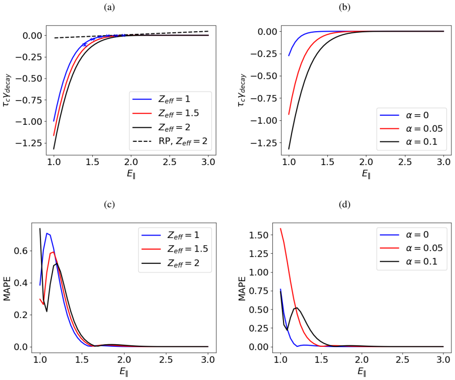
- [§IV B 2, Figs. 8–11] The inferred decay rates are based on a 20 τc trajectory with the last 5 τc used for exponential fits. The MAPE shown in Fig. 10 measures how well a decaying exponential fits the surrogate output, not how accurately the surrogate reproduces the kinetic solution. For electric fields well below threshold, the RE density is not well described by an exponential over this window (Fig. 8), so the fitted rates carry systematic uncertainty beyond the reported fitting error. The comparison with Ref. [44] covers only a subset of the parameter range. Please report confidence intervals for the decay rates, for example from multiple PINN training runs or from sensitivity to the fitting window, and state explicitly which portion of the decay-rate curve is quantitatively reliable.
minor comments (4)
- [§IV A, p. 15] The sentence saying that training-loss spikes are evident from Fig. 6(a) appears to refer to Fig. 4(a), since Fig. 6 contains RPF solutions rather than loss histories.
- [§IV B 2, p. 22] The MAPE values are described as percentages, but the example given as an MAPE of approximately 0.75 lacks a unit or percent sign; please clarify whether the maximum MAPE is 2% and whether 0.75 is 0.75% or a dimensionless value.
- [Abstract and §II B] The phrase "arbitrary initial momentum space distribution" is exact only for the mathematical projection in Eq. (14); for the trained surrogate it should be qualified to distributions within the trained parameter range and with adequate pointwise accuracy of P. Please adjust the wording to reflect the limitation stated in Section V.
- [Code availability, p. 14] The Python training script is promised upon acceptance; for a computational methods paper, providing the repository or supplementary code and data at the time of submission would strengthen reproducibility.
Circularity Check
No circular derivation: the PINN is trained on PDE residuals, not on the benchmark outputs; only minor same-group benchmark self-citations keep the score above zero.
full rationale
The core derivation is self-contained. The adjoint relation (Eqs. 5-10) is obtained by integration by parts from the relativistic Fokker-Planck equation, and Eq. (14), n_RE(t) = integral d^3p f_e^init P(p,xi,tau;t_final), is an exact projection of the density moment, not an ansatz or a fit. The PINN is trained with the loss in Eq. (19), which contains only the residual of the adjoint PDE and a soft upper-momentum-boundary term; no RAMc time histories or Ref. 44 decay rates enter the loss. Thus the headline comparisons with RAMc and with the decay-rate benchmarks are not fitted inputs renamed as predictions. The same-group provenance of RAMc (Refs. 7, 45) and of the decay-rate benchmarks (Ref. 44) is a minor self-citation issue: those benchmarks validate the surrogate's consistency with a traditional solver of the same kinetic equation, but they are not load-bearing for the derivation itself. Likewise, the companion paper [20] is cited for the large-angle-collision extension, but the primary-decay results and the comparison with Eq. (22) do not depend on it. The limitation explicitly flagged in Sec. V -- 'the modest accuracy that PINNs are able to achieve when solving a PDE in comparison to traditional Fokker-Planck solvers' and the fact that regions where P is nearly zero 'yield small contributions to the loss' -- is a genuine accuracy and scope caveat, visible in Fig. 12(c), but it concerns the reliability of deep-decay predictions rather than circularity. No uniqueness theorem, fitted parameter, or ansatz is imported from a same-author citation in a way that makes the central claim equivalent to its inputs by construction.
Assumptions & free parameters
free parameters (6)
- p_RE runaway momentum cutoff =
p_RE = p_max/4 (about 1 MeV)
- Delta_p terminal smoothing width =
0.1 p_max
- Delta_P magnitude =
0.15
- t_final adjoint horizon =
20 tau_c (one run with 40 tau_c)
- w_PDE loss weight =
10
- Delta_p_max boundary-weight width =
0.05 p_max
assumptions (6)
- domain assumption Relativistic Fokker-Planck operator with electric field acceleration, small-angle collisions, and synchrotron radiation
- domain assumption Energy diffusion is negligible
- domain assumption Completely screened Coulomb collision operator
- standard math Adjoint integration by parts with only the upper momentum boundary flux surviving
- domain assumption Cold bulk: electrons crossing p_min are absorbed and never re-enter
- ad hoc to paper The PINN optimization converges to the PDE solution on the training domain
Cite this review
Pith. "Pith review of A Physics-Constrained Deep Learning Treatment of Runaway Electron Dynamics." pith.science (2026). https://pith.science/paper/ATWPM4LN
@misc{pith2026241212980,
  author       = {Pith},
  title        = {Pith review of: A Physics-Constrained Deep Learning Treatment of Runaway Electron Dynamics},
  year         = {2026},
  howpublished = {\url{https://pith.science/paper/ATWPM4LN}},
  note         = {Machine review of arXiv:2412.12980}
}
read the original abstract
An adjoint formulation leveraging a physics-informed neural network (PINN) is employed to advance the density moment of a runaway electron (RE) distribution forward in time. A distinguishing feature of this approach is that once the adjoint problem is solved, its solution can be used to project the RE density forward in time for an arbitrary initial momentum space distribution of REs. Furthermore, by employing a PINN, a parametric solution to the adjoint problem can be learned. Thus, once trained, this adjoint-deep learning framework is able to efficiently project the RE density forward in time across various plasma conditions while still including a fully kinetic description of RE dynamics. As an example application, the temporal evolution of the density of primary electrons is studied, with particular emphasis on evaluating the decay of a RE population when below threshold. Predictions from the adjoint-deep learning framework are found to be in good agreement with a traditional relativistic electron Fokker-Planck solver, for several distinct initial conditions, and across an array of physics parameters. Once trained the PINN thus provides a means of generating RE density time histories with exceptionally low online execution time.
Figures


Figures from the paper (9 more)




Reference graph
Works this paper leans on
-
[44]
F. Andersson, P. Helander, and L.-G. Eriksson, Physics of Plasmas 8, 5221 (2001)
work page 2001
-
[1]
IV A to evaluate the time history of the RE densitynRE using Eq
Time Histories of RE Density for Different Initial Conditions In this section we will utilize the parametric solution to the time dependent RPF described in Sec. IV A to evaluate the time history of the RE densitynRE using Eq. (14). Taking the initial RE population to be of the form: f (init) e (p, ξ) ∝ exp " − (p − p0)2 ∆p2 − (ξ − ξ0)2 ∆ξ2 # , (21) the t...
-
[2]
Using a RE decay rate to characterize RE evolution comes with two significant caveats
Runaway Electron Decay Rate The time evolution of the RE density can be used to estimate the decay rate of a primary electron population when below threshold. Using a RE decay rate to characterize RE evolution comes with two significant caveats. The first is that while the RE density exhibits an exponential decay when 19 (a) (b) Figure 8. The time evoluti...
-
[3]
P. C. De Vries, Y . Lee, Y . Gribov, A. Mineev, Y . Na, R. Granetz, B. Stein-Lubrano, C. Reux, P. Moreau, V . Kiptily, et al., Nuclear Fusion63, 086016 (2023)
work page 2023
-
[4]
Hender, J
T. Hender, J. Wesley, J. Bialek, A. Bondeson, A. Boozer, R. Buttery, A. Garofalo, T. Goodman, R. Granetz, Y . Gribov, et al., Nuclear fusion47, S128 (2007)
2007
-
[5]
B. N. Breizman, P. Aleynikov, E. M. Hollmann, and M. Lehnen, Nuclear Fusion 59, 083001 (2019)
2019
-
[6]
Nilsson, J
E. Nilsson, J. Decker, Y . Peysson, R. S. Granetz, F. Saint-Laurent, and M. Vlainic, Plasma Physics and Controlled Fusion 57, 095006 (2015)
2015
- [7]
Show all 51 references
-
[8]
Harvey, V
R. Harvey, V . Chan, S. Chiu, T. Evans, M. Rosenbluth, and D. Whyte, Physics of Plasmas 7, 4590 (2000)
2000
-
[9]
Beidler, D
M. Beidler, D. del Castillo-Negrete, D. Shiraki, L. R. Baylor, E. M. Hollmann, and C. Lasnier, Nuclear Fusion 64, 076038 (2024)
2024
-
[10]
C. J. McDevitt, Z. Guo, and X. Z. Tang, Plasma Physics and Controlled Fusion 61, 054008 (2019)
2019
-
[11]
Hoppe, O
M. Hoppe, O. Embreus, and T. F ¨ul¨op, Computer Physics Communications 268, 108098 (2021)
2021
-
[12]
Sainterme and C
A. Sainterme and C. Sovinec, Physics of Plasmas 31 (2024)
2024
-
[13]
Bandaru, M
V . Bandaru, M. Hoelzl, C. Reux, O. Ficker, S. Silburn, M. Lehnen, N. Eidietis, J. Contributors, J. Team, et al., Plasma Physics and Controlled Fusion 63, 035024 (2021)
2021
-
[14]
C. Liu, C. Zhao, S. C. Jardin, N. M. Ferraro, C. Paz-Soldan, Y . Liu, and B. C. Lyons, Plasma Physics 28 and Controlled Fusion 63, 125031 (2021)
2021
-
[15]
M. Yang, P. Wang, D. del Castillo-Negrete, Y . Cao, and G. Zhang, SIAM Journal on Scientific Com- puting 46, C508 (2024)
2024
-
[16]
H. M. Smith and E. Verwichte, Physics of plasmas 15, 072502 (2008)
2008
-
[17]
C. J. McDevitt, Physics of Plasmas 30, 092501 (2023), ISSN 1070-664X, URL https://doi. org/10.1063/5.0164712
2023 doi
-
[18]
Hesslow, O
L. Hesslow, O. Embr ´eus, O. Vallhagen, and T. F¨ul¨op, Nuclear Fusion 59, 084004 (2019)
2019
-
[19]
SOKOLOV , JETP Letters29, 218 (1979)
I. SOKOLOV , JETP Letters29, 218 (1979)
1979
-
[20]
Rosenbluth and S
M. Rosenbluth and S. Putvinski, Nuclear Fusion 37, 1355 (1997)
1997
-
[21]
C. F. Karney and N. J. Fisch, The Physics of fluids 29, 180 (1986)
1986
-
[22]
J. S. Arnaud, T. Mark, and C. J. McDevitt, J. Plasma Phys. 90, 905900409 (2024)
2024
-
[23]
McDevitt et al., An efficient surrogate model of secondary electron dynamics, Submitted to Physics of Plasmas (2024)
C. McDevitt et al., An efficient surrogate model of secondary electron dynamics, Submitted to Physics of Plasmas (2024)
2024
-
[24]
Raissi, P
M. Raissi, P. Perdikaris, and G. E. Karniadakis, Journal of Computational physics 378, 686 (2019)
2019
-
[25]
C. Liu, D. P. Brennan, A. H. Boozer, and A. Bhattacharjee, Plasma Physics and Controlled Fusion 59, 024003 (2017), URL http://stacks.iop.org/0741-3335/59/i=2/a=024003
2017
-
[26]
Zhang and D
G. Zhang and D. del Castillo-Negrete, Physics of Plasmas 24, 092511 (2017)
2017
-
[27]
L. Sun, H. Gao, S. Pan, and J.-X. Wang, Computer Methods in Applied Mechanics and Engineering 361, 112732 (2020)
2020
-
[28]
G. E. Karniadakis, I. G. Kevrekidis, L. Lu, P. Perdikaris, S. Wang, and L. Yang, Nature Reviews Physics 3, 422 (2021)
2021
-
[29]
S. Cai, Z. Mao, Z. Wang, M. Yin, and G. E. Karniadakis, Acta Mechanica Sinica 37, 1727 (2021)
2021
-
[30]
Taguchi, Journal of the Physical Society of Japan 52, 2035 (1983)
M. Taguchi, Journal of the Physical Society of Japan 52, 2035 (1983)
1983
-
[31]
C. J. McDevitt and X.-Z. Tang, Physics of Plasmas 31 (2024)
2024
-
[32]
Antonsen Jr and K
T. Antonsen Jr and K. Chu, The Physics of Fluids 25, 1295 (1982)
1982
-
[33]
Connor and R
J. Connor and R. Hastie, Nuclear fusion 15, 415 (1975)
1975
-
[34]
Fisch, The Physics of fluids 29, 172 (1986)
N. Fisch, The Physics of fluids 29, 172 (1986)
1986
-
[35]
C. Liu, D. P. Brennan, A. Bhattacharjee, and A. H. Boozer, Physics of Plasmas 23, 010702 (2016)
2016
-
[36]
Lusch, J
B. Lusch, J. N. Kutz, and S. L. Brunton, Nature communications 9, 1 (2018)
2018
-
[37]
I. E. Lagaris, A. Likas, and D. I. Fotiadis, IEEE transactions on neural networks 9, 987 (1998)
1998
-
[38]
Karpatne, G
A. Karpatne, G. Atluri, J. H. Faghmous, M. Steinbach, A. Banerjee, A. Ganguly, S. Shekhar, N. Sam- 29 atova, and V . Kumar, IEEE Transactions on knowledge and data engineering29, 2318 (2017)
2017
-
[39]
Abadi, P
M. Abadi, P. Barham, J. Chen, Z. Chen, A. Davis, J. Dean, M. Devin, S. Ghemawat, G. Irving, M. Isard, et al., in 12th USENIX symposium on operating systems design and implementation (OSDI
-
[40]
(b) Projection of the final training point distribution onto the energy and pitch domain
every 50,000 epochs of L-BFGS. (b) Projection of the final training point distribution onto the energy and pitch domain. parameters will be considered in Ref. [20]. We have also chosen a domain with a minimum energy of 10 keV, a maximum energy of5 MeV, and tf inal= 20. The ene...
-
[41]
R. Wang, K. Kashinath, M. Mustafa, A. Albert, and R. Yu, in Proceedings of the 26th ACM SIGKDD International Conference on Knowledge Discovery & Data Mining (2020), pp. 1457–1466
2020
-
[42]
L. Lu, X. Meng, Z. Mao, and G. E. Karniadakis, SIAM Review 63, 208 (2021)
2021
-
[43]
C. Wu, M. Zhu, Q. Tan, Y . Kartha, and L. Lu, Computer Methods in Applied Mechanics and Engi- neering 403, 115671 (2023)
2023
-
[45]
Decker, E
J. Decker, E. Hirvijoki, O. Embreus, Y . Peysson, A. Stahl, I. Pusztai, and T. F ¨ul¨op, Plasma Physics and Controlled Fusion 58, 025016 (2016)
2016
-
[46]
Z. Guo, C. J. McDevitt, and X.-Z. Tang, Plasma Physics and Controlled Fusion 59, 044003 (2017)
2017
-
[47]
C. J. McDevitt, Z. Guo, and X.-Z. Tang, Plasma Physics and Controlled Fusion 60, 024004 (2018)
2018
-
[48]
McDevitt and X.-Z
C. McDevitt and X.-Z. Tang, EPL (Europhysics Letters) 127, 45001 (2019)
2019
-
[49]
B. N. Breizman, Nuclear Fusion 54, 072002 (2014)
2014
-
[50]
C. J. McDevitt and X.-Z. Tang, Physical Review E 108, L043201 (2023)
2023
-
[51]
Hesslow, O
L. Hesslow, O. Embr ´eus, A. Stahl, T. C. DuBois, G. Papp, S. L. Newton, and T. F ¨ul¨op, Phys. Rev. Lett. 118, 255001 (2017), URL https://link.aps.org/doi/10.1103/PhysRevLett. 118.255001. 30
2017 doi
Reviewed August 11, 2026 · model on record in the stance chip above.
Discussion (0). Continue with ORCID to comment.