REVIEW 4 major objections 6 minor 5 references
Reaching the equilibrium: Long-term stable approximations for stochastic non-Newtonian Stokes equations with transport noise
T0 review · 4 major / 6 minor · reviewed 2026-08-11 · deepseek-v4-flash
Pith's one-line read Constructs a long-term stable, fully discrete scheme for the stochastic non-Newtonian Stokes equations and uses it to build approximate invariant measures, with the zero-boundary equilibrium shown to be the Dirac mass at zero.
desk verdict Honest, technically strong paper whose real results are the time-uniform stability theorem and the discrete invariant-measure machinery; the general-boundary existence claim is conditional on a condition the authors expect to fail. read the letter →
The pith
A machine-rendered reading of the paper's core claim, the machinery that carries it, and where it could break.
The reading
What carries the argument
The engine of the construction is the pair consisting of a Gradient Discretisation in space and a semi-implicit Crank-Nicolson step in time. A Gradient Discretisation packages a spatial scheme through reconstruction operators; the paper requires a Γ-stable family in which coercivity, inf-sup stability, and the Sobolev stability of the L2-projection onto the discrete divergence-free space are uniformly controlled. The transport noise is discretised through Temam's symmetrisation, B^σ_D(v,ξ)=1/2(σ^T∇_D v, Π_D ξ)−1/2(Π_D v, σ^T∇_D ξ), which is skew-symmetric and vanishes on the diagonal, so the noise term cancels in the discrete energy balance. The proof of Theorem 11 then sums local energy inequalities, converts dissipation into Lp control of the symmetric gradient via the relation S(A):(A−B) ≂ |V(A)−V(B)|^2, and absorbs stochastic terms using the Burkholder-Davis-Gundy inequality.
What would settle it
Choose a sequence of increasingly refined mixed finite-element discretisations of the divergence-free Stokes problem and compute C^Sob_D(p)+C^Sob_D(p') on the discrete divergence-free subspace; if these constants grow without bound, the proof of Theorem 11 fails at the noise estimate Term II. Alternatively, fix τ and estimate the time-averaged mean squared velocity increment E[(1/N) Σ_ℓ ||Π_D $v^{{ℓ+1}}$_D − Π_D v^ℓ_D||^2] for large N; the numerical results suggest it tends to a positive τ-dependent constant rather than zero, which would violate condition (4.2) and block the invariance of the second measure sequence for fixed τ.
Extended reading notes
Core claim
The central discovery is that a Crank-Nicolson time discretisation combined with a Gradient Discretisation in space reproduces, on the discrete level, the energy dissipation mechanism that makes transport noise special: the noise term is discretised by a skew-symmetric bilinear form that vanishes on its diagonal, so it drops out of the discrete energy identity. This yields a pathwise energy equality for zero boundary data and an energy inequality with only linear growth in the horizon for general Dirichlet data. From that stability the paper derives a discrete Markov semigroup, proves it has at most one invariant measure, and identifies two constructor sequences: an ergodic-average sequence that is asymptotically invariant to order n/N, and a shifted-average sequence that is tight and therefore has a limit measure. A condition on the time-averaged squared velocity increment merges the two properties, and the authors show it holds in the trivial-boundary case, where the unique invariant measure is δ0 and both sequences converge to it.
Load-bearing premise
The proof of the main stability theorem requires the L2-projection onto the discretely divergence-free velocity space to be uniformly Sobolev-stable, meaning bounded by a fixed constant across the whole family of discretisations; the paper itself notes that this property has not been verified for constrained divergence-free subspaces. If this constant blows up under mesh refinement, the time-uniform estimate, the tightness of the second measure sequence, and hence the invariant-measure construction would no longer follow.
Editorial extensions
If this is right
- For every moment q>0, discrete solutions satisfy a time-uniform bound growing only linearly in the horizon, so simulations can be run to arbitrarily long times without blow-up.
- The discrete transition semigroup has at most one invariant measure, so any successfully constructed stationary distribution is the unique equilibrium of the discrete dynamics.
- The empirical measure sequence (4.1a) is asymptotically invariant with an O(n/N) discrepancy, meaning any weak limit point of that sequence is invariant for the discrete semigroup.
- The shifted sequence (4.1b) is tight and therefore has a weak limit measure for fixed discretisation parameters and also in various joint refinement regimes, provided the analytic horizon stays non-degenerate.
- For homogeneous boundary data g=0, the unique invariant measure is δ0 and both measure sequences converge to it, characterising the equilibrium completely in that case.
Reading between the lines
- If condition (4.2) indeed fails for fixed τ, as the numerical results suggest, then for a fixed discretisation one should not expect a stationary distribution at integer times; the authors' planned route through a time-continuous limit is then the natural way to obtain an invariant measure.
- The pathwise energy equality for zero boundary data makes the scheme a candidate for unbiased sampling of the trivial equilibrium: because energy dissipates monotonically along each trajectory, burn-in can be monitored deterministically rather than statistically.
- A direct test of the paper's main assumption would be to compute the Sobolev-stability constant of the L2-projection onto the discrete divergence-free space on a sequence of refined meshes; if it grows without bound, the uniform Γ-stability needed by Theorem 11 cannot be verified empirically for refined families.
- The implemented algorithm already accommodates an external deterministic force and non-solenoidal boundary data; extending the invariant-measure analysis to that setting would give a nontrivial limit measure, unlike the δ0 obtained for homogeneous data.
Editorial analysis
A structured set of objections, weighed in public.
Referee Report
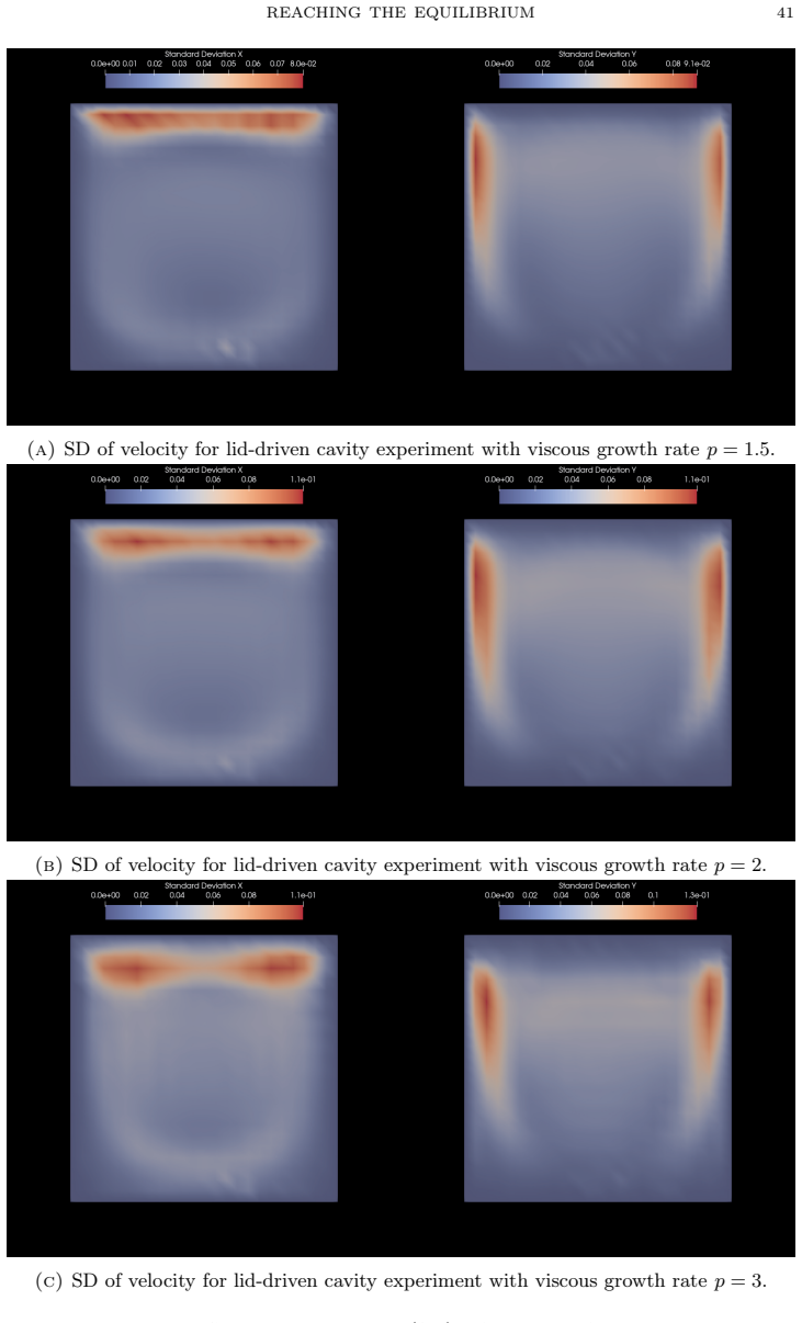
Summary. The paper proposes a fully discrete numerical scheme for the generalised Stokes system driven by transport noise, based on the Gradient Discretisation Method and a Crank--Nicolson-type time stepping with Temam's antisymmetric noise discretisation. Under a set of structural assumptions on the gradient discretisation (Assumption 10), it proves long-term stability of the scheme with constants growing at most linearly in the time horizon (Theorem 11), establishes at most one invariant measure for the discrete transition semigroup (Theorem 18), and constructs two sequences of empirical measures with complementary properties: the first is asymptotically invariant (Lemma 19) and the second has a tightness-based limit (Lemma 21). A sufficient condition (4.2) is given to merge existence and invariance, and the homogeneous-boundary case is fully characterised by convergence to the Dirac measure at zero (Example 25). Two numerical experiments on Taylor--Hood elements illustrate the influence of transport noise on dissipation, mixing, and vortex structure, and investigate the validity of condition (4.2).
Significance. If the results are fully correct, this is the first work to construct computable approximations of invariant measures for stochastic non-Newtonian Stokes equations with transport noise, a genuinely new contribution to the numerical SPDE literature. The paper's strengths include the transparent tracking of all constants, the elegant diagonal-vanishing antisymmetric noise discretisation that preserves discrete energy cancellation, the fully written proofs of the main stability and uniqueness theorems, and the honest and explicit discussion of the remaining gaps (Remark 9, Remark 24, Section 7). The numerical experiments are reproducible in principle through the linked Firedrake-based code and directly probe the paper's central abstract condition. However, the advertised 'broad class' of gradient discretisations is not actually demonstrated: the uniform Sobolev-stability of the L2-projection onto discretely divergence-free subspaces (Assumption 10) is unverified for any family of discretisations, and the semigroup property -- essential for the invariant measure framework -- is only proved informally.
major comments (4)
- [Section 3.1, Assumption 10, Definition 8, Eq. (3.5); proof of Theorem 11, Eq. (5.6)] The uniform Sobolev-stability assumption on the L2-projection onto the discretely divergence-free subspace is the key structural condition that makes the time-global stability estimate (3.9) independent of the spatial discretisation. It enters the proof of Theorem 11 through the constant K = Gamma^3 ||sigma||_Linf ||(sigma . grad) g||_{W^{1,p'}} in the estimate of Term II in (5.6); without uniformity in the discretisation family, (3.9) carries a mesh-dependent constant, and the tightness argument in Lemma 21 loses the uniformity needed to produce a limit measure. The authors explicitly state in Remark 9 that stability for constrained subspaces such as E_{D,0} 'remains to be explored'. As it stands, no example of a Gradient Discretisation family satisfying Assumption 10 is provided, so the claim of long-term stability for a broad class of particular GDs is not supported by any concrete family. The manuscript should either supply such a family (for instance by verifying the assumption for Taylor--Hood elements under mesh refinement) or relax the assumption and show which parts of the theory survive without it.
- [Section 5.2.1, Lemma 15] The semigroup property of P_{tau,D} is foundational: it justifies calling P_{tau,D} a discrete transition semigroup, is used in the definition of an invariant measure, and underpins the uniqueness theorem (Theorem 18) and the asymptotic invariance estimate (Lemma 19). However, the proof of Lemma 15 is only informal: it states 'We provide an informal argument only' and defers the rigorous justification to a limit passage over finite sums that is never carried out. In particular, the representation S(n,v_in) = S^{diamond n}_{CN}[K_D v_in, Delta_1 W, ..., Delta_n W] and the use of continuity in the random update (Lemma 31) require a careful treatment of the measurability and approximation steps. This gap must be closed before the invariant measure construction can be considered complete.
- [Section 6.3, Eq. (6.1); Section 4.2, Eq. (4.2), Figure 1, Table 1] The numerical experiments are performed with a 'slightly modified' scheme that includes an external deterministic force F and, in EXP-2, non-solenoidal boundary data g, while the theoretical analysis of Theorem 11 and the energy identities are established for the scheme (3.8) under Assumption 1, which requires g to be solenoidal and uses the shift v = u - g. The modified scheme (6.1) is not shown to satisfy the structural properties used in the analysis (for example, the diagonal cancellation of the noise term after the shift, or the pathwise energy identity for g=0). Consequently, the numerical conclusion that condition (4.2) fails in general (Figure 1, Table 1) is not direct evidence about the analysed scheme. The authors should either prove that the modified scheme inherits the relevant structural properties or reformulate the numerical investigation so that it tests the analysed scheme.
- [Section 4.2, condition (4.2); Example 25] The only general-boundary result that yields existence of an invariant measure is the abstract condition (4.2), and the only example where it is verified is the trivial-boundary case g = 0 (Example 25), where the invariant measure is delta_0. For nontrivial g, no example satisfying (4.2) is given, and the numerical evidence suggests that the condition may fail for small time steps. The paper is honest about this, but the advertised 'recovering the existence of an invariant measure' is thus a conditional statement without a nontrivial instantiation. It would considerably strengthen the paper to provide a nontrivial class of data for which (4.2) can be verified, or at least a precise discussion of why such a class is expected to be empty or nonempty.
minor comments (6)
- [Definition 2(f)] The definition of Y_{D,0} is self-referential: it reads 'Y_{D,0} = {q in Y_{D,0} : ...}'. The right-hand side should use the full space Y_D or a different symbol for the mean-free subspace.
- [Remark 22] The labels in the bullet list appear swapped: the third bullet says 'space discrete case (D fixed, tau -> 0 and N -> infinity such that tau N >= 1)', which is a time-discrete case, while the fourth bullet describes the fully continuous limit. The terminology should be corrected.
- [Proof of Lemma 21] The set D_R is defined as all L2 vector fields of the form Pi_D v_D with ||epsilon_D v_D||_{L^p} <= R, and is claimed to be compact. Strictly, D_R as defined may not be closed; for the tightness argument one can take its closure, which is compact because it is a bounded subset of the finite-dimensional space Pi_D X_{D,0}. This detail should be stated.
- [Section 6.4, EXP-1] The phrase 'the stochastic velocity vector points in all directions with positive probability' is a strong statement about the support of the stationary distribution at a fixed point; the numerical evidence is only based on a finite sample and finite-time observations, so this should be phrased as an observation rather than an established fact.
- [Section 5.1, proof of Theorem 11] In the estimate of R3, the martingale increments are centred and the quadratic variation is handled correctly, but the notation 'N0 ∋ M' is unusual; this is a minor stylistic point.
- [Section 2.5] The formal energy inequality (2.4) uses the Helmholtz--Leray projection P in the Itô--Stratonovich corrector, but the corrector term is not fully derived; a reference or a couple of additional lines would help the reader. Since this is only motivation, the informal derivation is acceptable.
Circularity Check
No circular reasoning detected: the long-term stability and invariant-measure results are derived from explicit assumptions and energy estimates, with the paper's own flagged limitations pointing to generality gaps rather than circularity.
full rationale
The derivation chain is self-contained. Theorem 11's long-term stability bound (3.9) follows from the discrete energy identity (5.3), the tensor equivalence of Lemma 26, the generalized Young inequality (5.2), the antisymmetry of B^σ_D (which makes the noise term vanish on the diagonal), and martingale estimates; Assumption 10 enters only as a stated hypothesis through explicit constants such as K = Γ^3 ||σ||_L∞ ||(σ·∇)g||_{W^{1,p'}} in (5.6), not as a fitted parameter or as a re-statement of the conclusion. The tightness of the second measure sequence (Lemma 21) uses exactly the time-uniform bound (3.9) and the finite-dimensionality of Π_D X_{D,0}, not a pre-supposed invariant measure. Lemma 19's asymptotic invariance is a Cesàro telescoping identity (5.33), independent of any measure existence. Theorem 18's uniqueness is proved from a pathwise two-solution energy equivalence (5.27) and Lemma 32, not imported from the authors' prior work. Example 25's characterization of the invariant measure as δ_0 follows from the pathwise energy equality (3.10) plus the proved uniqueness. Self-citations such as [DGL22], [DKL24], [LW24], and [Wic24] are contextual or relate to prior methods and do not carry a load-bearing step here. The paper explicitly flags its weakest point: Remark 9 states that Sobolev-stability of the L2-projection on constrained subspaces such as E_{D,0} 'remains to be explored', which is an honest limitation on the breadth of Assumption 10 rather than a circular step; similarly, the numerics in Table 1 show that the sufficient condition (4.2) fails for fixed τ, which is the opposite of forcing the abstract condition. No fitted input is renamed as a prediction, and no known result is repackaged as new.
Assumptions & free parameters
assumptions (6)
- domain assumption Data conditions: g in W^{2,inf}_div, sigma in W^{1,inf}_div, vin in L2 (Assumption 1)
- domain assumption Gamma-stability of the GD: uniform bounds on coercivity, inf-sup and Sobolev-stability constants (Assumption 10)
- standard math Well-posedness of each nonlinear time step via monotone operator theory and the Banach-Necas-Babuska theorem
- standard math Tensor inequalities (Lemmas 26, 27, 32) cited from [DE08], [DFTW20] and [BDR08]
- standard math Stochastic calculus toolkit: Stratonovich-to-Ito conversion, Burkholder-Davis-Gundy inequality, Gaussian moment bounds
- ad hoc to paper The numerically implemented 'slightly modified' scheme (external force F, non-solenoidal lid g) obeys the same structural properties as the analysed scheme
invented entities (1)
-
Antisymmetric noise discretisation B_sigma_D (Temam device) and shifted-integer time scale
independent evidence
Cite this review
Pith. "Pith review of Reaching the equilibrium: Long-term stable approximations for stochastic non-Newtonian Stokes equations with transport noise." pith.science (2026). https://pith.science/paper/6UG2BHSX
@misc{pith2026241214316,
  author       = {Pith},
  title        = {Pith review of: Reaching the equilibrium: Long-term stable approximations for stochastic non-Newtonian Stokes equations with transport noise},
  year         = {2026},
  howpublished = {\url{https://pith.science/paper/6UG2BHSX}},
  note         = {Machine review of arXiv:2412.14316}
}
read the original abstract
We propose and analyse a novel, fully discrete numerical algorithm for the approximation of the generalised Stokes system forced by transport noise -- a prototype model for non-Newtonian fluids including turbulence. Utilising the Gradient Discretisation Method, we show that the algorithm is long-term stable for a broad class of particular Gradient Discretisations. Building on the long-term stability and the derived continuity of the algorithm's solution operator, we construct two sequences of approximate invariant measures. At the moment, each sequence lacks one important feature: either the existence of a limit measure, or the invariance with respect to the discrete semigroup. We derive an abstract condition that merges both properties, recovering the existence of an invariant measure. We provide an example for which invariance and existence hold simultaneously, and characterise the invariant measure completely. We close the article by conducting two numerical experiments that show the influence of transport noise on the dynamics of power-law fluids; in particular, we find that transport noise enhances the dissipation of kinetic energy, the mixing of particles, as well as the size of vortices.
Figures


Figures from the paper (6 more)




Reference graph
Works this paper leans on
-
[140]
The Gradient Discretization Method for Slow and Fast Diffusion Porous Media Equations
doi: 10.1016/j.camwa.2024.08.007. [DL20] J. Droniou and K.-N. Le. “The Gradient Discretization Method for Slow and Fast Diffusion Porous Media Equations”. In:SIAM Journal on Numerical Analysis58.3 (Jan. 2020), pp. 1965–1992.doi: 10.1137/19m1260165. [EŠ17] E. Emmrich and D. Šiška. “Nonlinear stochastic evolution equations of second order with damping”. In:...
-
[244]
doi: 10.1007/s00032-009-0100-0. [KHH18] M. Kamrani, S. M. Hosseini, and E. Hausenblas. “Implicit Euler method for numerical solution of nonlinear stochastic partial differential equations with multiplicative trace class noise”. In:Math. Methods Appl. Sci.41.13 (2018), pp. 4986–5002.doi: 10.1002/ mma.4946. [KV24] K.KliobaandM.Veraar.“Pathwiseuniformconverg...
-
[260]
doi: 10.1007/s10543-006-0062-3. [Bon+21] F. Bonaldi et al. “Gradient discretization of two-phase poro-mechanical models with discontinuouspressuresatmatrixfractureinterfaces”.In: ESAIM: Mathematical Mod- elling and Numerical Analysis55.5 (Sept. 2021), pp. 1741–1777.doi: 10.1051/m2an/ 2021036. [BDD19] L. Botti, D. A. Di Pietro, and J. Droniou. “A Hybrid Hi...
arXiv 2021
-
[1032]
The Numerical Approximation of Stochastic Partial Differential Equations
doi: 10.4007/annals.2006.164.993. [Ham+23] D. A. Ham et al. Firedrake User Manual. First edition. Imperial College London et al. May 2023. doi: 10.25561/104839. [JK09] A. Jentzen and P. E. Kloeden. “The Numerical Approximation of Stochastic Partial Differential Equations”. In:Milan Journal of Mathematics77.1 (Sept. 2009), pp. 205–
-
[2607]
Numerical and convergence analysis of the stochastic Lagrangian averaged Navier–Stokes equations
doi: 10.1137/20m1358013. [DG22] J. Doghman and L. Goudenège. “Numerical and convergence analysis of the stochastic Lagrangian averaged Navier–Stokes equations”. In:Journal of Computational and Applied Mathematics414 (Nov. 2022), p. 114446.doi: 10.1016/j.cam.2022.114446. [DEF15] J. Droniou, R. Eymard, and P. Feron. “Gradient Schemes for Stokes problem”. In...
Reviewed August 11, 2026 · model on record in the stance chip above.
Discussion (0). Continue with ORCID to comment.