REVIEW 2 major objections 4 minor 2 cited by
A random walk among random graphs
T0 review · 2 major / 4 minor · reviewed 2026-08-10 · deepseek-v4-flash
Pith's one-line read These master lecture notes contend that a handful of probabilistic tools—random-walk encodings, moment methods, exploration processes, and continuous-time embeddings—gives a unified route through random graphs, branching trees, and random…
desk verdict Lecture notes, not research: solid pedagogical value, but the Wiener–Hopf sign inconsistency and unresolved placeholders need fixing before publication. read the letter →
The pith
A machine-rendered reading of the paper's core claim, the machinery that carries it, and where it could break.
The reading
What carries the argument
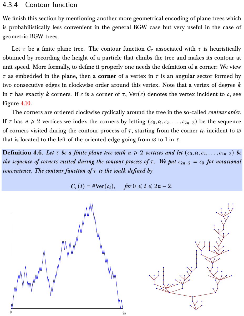
The central object is the Łukasiewicz walk: for a plane tree, list vertices in breadth-first order and take steps equal to (#children − 1). This turns a tree into a skip-free random walk, so the cycle lemma, Kemperman's formula, and ballot theorems compute tree counts, hitting times, and extinction probabilities. For G(n,p), the corresponding tool is the exploration process (stack, untouched, and explored vertices), a Markov chain with Binomial increments that converges, via the differential-equation method, to the fluid limit f_c. Continuous-time Yule trees and spinal decomposition play the same unifying role for random recursive and preferential-attachment trees.
What would settle it
Simulate the exploration of G(n,c/n) for c=0.8, 1, and 1.2 with n=$10^{5}$, and compare the empirical largest-component fraction and the number of components with the predicted values 1−α(c) and n·α(c)(2−cα(c))/2; if they do not converge to these quantities, the fluid-limit derivation of Chapter 7 is wrong.
Extended reading notes
Core claim
The paper's central claim is didactic: a reader who masters a compact set of probabilistic techniques can derive the main theorems of random graph theory rather than taking them on faith. The key reduction is the Łukasiewicz walk, which encodes a plane tree as a skip-free random walk, making Feller's cycle lemma and Kemperman's formula available for enumeration and hitting-time problems. The same walk appears as the exploration process of the Erdős–Rényi graph G(n,p), whose increments are Binomial; a fluid-limit argument shows the rescaled exploration converges to a deterministic function f_c, from which the giant-component phase transition at c=1 and the logarithmic bounds on smaller components follow. The notes extend the method to random permutations through Feller coupling, to random recursive trees through the Chinese restaurant process and Pólya urns, and to Barabási–Albert trees through Yule-process embedding and spinal decomposition.
Load-bearing premise
The course presupposes a reader already comfortable with measure-theoretic probability, martingales, and Fourier analysis, and it imports deep external theorems without proof, such as the local central limit theorem and the Aldous–Le Gall convergence to the Brownian continuum random tree; if any of those external results is misstated or the reader lacks the background, the self-contained pedagogical promise collapses.
Editorial extensions
If this is right
- For G(n,c/n) with c<1, all connected components have size O(log n) with high probability; for c>1, a unique giant component carries fraction 1−α(c) of the vertices and the second-largest component has size O(log n).
- The number of connected components of G(n,c/n) divided by n converges to α(c)(2−cα(c))/2, where α(c) solves α=e^{-c(1−α)}.
- Plane trees with prescribed out-degrees are counted by (n−1)!/∏ d_i!, and the Catalan numbers count plane trees; both follow from the Łukasiewicz walk and the cycle lemma.
- A uniform plane tree's typical height, after normalization by √n, converges to a Rayleigh law, and the same limit holds for uniform Cayley trees.
- The random recursive tree has height of order e log n and maximal degree of order log n/log log n, while the Barabási–Albert tree has a power-law degree distribution with exponent 3.
Reading between the lines
- The exploration–fluid-limit scheme shown for G(n,p) is generic: for stochastic block models or configuration models, the same Markov exploration with different increment distributions should yield coupled ODE limits and giant-component thresholds, a route the notes only gesture at.
- The cycle-lemma/Kemperman-formula engine that produces parking-function probabilities and tree counts is likely to give distributional results for cluster sizes in the critical Erdős–Rényi window by conditioning the same random walks.
- The three proofs of the giant component form a hierarchy: the ε-cut proof establishes the density but not the logarithmic bounds, the exploration proof refines it, and the Poissonized version smooths the critical window; this hierarchy is a transferable template for proving phase transitions in other random graph models.
Editorial analysis
A structured set of objections, weighed in public.
Referee Report
Summary. The manuscript is a set of lecture notes from a master course, covering one-dimensional random walks and skip-free walks, the cycle lemma and Wiener–Hopf factorization, Bienaymé–Galton–Watson trees and their Łukasiewicz encodings, local properties of Erdős–Rényi graphs, three proofs of the giant-component phase transition, random permutations, random recursive trees, continuous-time embeddings, spine decompositions, and the Barabási–Albert preferential attachment tree. The stated goal in the introduction is to give a glimpse of several random-graph models together with the probabilistic tools used to study them, at the master/PhD level, rather than to provide an authoritative reference. The notes contain many worked examples, exercises, historical remarks, and explicit pointers to the literature.
Significance. If corrected, the notes would fulfill their stated pedagogical goal: they present a coherent selection of standard material with several detailed proofs, including the Łukasiewicz encoding, Kemperman's formula, and the exploration-process proof of the giant component. The multiple proofs of the emergence of the giant component and the explicit computations of Borel–Tanner and Catalan laws are notable strengths. No new research theorem is claimed, so the natural standard of assessment is internal correctness and pedagogical clarity. By that standard the manuscript is not yet ready, because one load-bearing tool section contains an unresolved sign inconsistency and the draft contains unresolved placeholders; these issues can be fixed locally, and the rest of the exposition is largely sound.
major comments (2)
- [§3.4.2, Theorem 3.12 and Remark 3.4] The sign conventions in the Wiener–Hopf factorization are inconsistent. The second display of Theorem 3.12 asserts 1 − E[r^{T_1^≤} e^{μ H_1^≤}] = exp(−Σ_n r^n/n E[e^{μ S_n} 1_{S_n≤0}]), while Remark 3.4 defines ω_r^≤(μ) with e^{−μ S_n} on the same event and then states the factorization ω_r^>(it) ω_r^≤(it) = 1 − r E[e^{−it X_1}] in (3.7). With the theorem's displayed factors, setting μ = it gives e^{−it S_n} on {S_n > 0} and e^{+it S_n} on {S_n ≤ 0}, so the product is not 1 − r E[e^{−it X_1}]. Because the proof derives only the first display and says the second is “similar”, a reader cannot resolve the discrepancy from the text. This is load-bearing for a central tool in Part I and needs correction: either the second display, the definition in Remark 3.4, or the identity (3.7) must be changed consistently.
- [§3.4.2, proof of Theorem 3.12] The statement “the calculation is similar for the second one” is not sufficient once the displayed signs disagree with the surrounding definitions. Even if the intended version is the standard Spitzer–Baxter formula, the manuscript should either prove the second display with the exact conventions used, or state both factors through a common convention and verify the product identity (3.7) explicitly. As written, the gap is not merely cosmetic: it prevents the reader from using the theorem to reproduce the factorization in Remark 3.4.
minor comments (4)
- [Notations] In the definition of [z^n] f(z), the text writes f(z) = Σ_{i≥0} f_i z^i ∈ C[[X]]; the ring should be C[[z]], since the indeterminate is z rather than X.
- [Corollary 3.2] In the proof of Corollary 3.2, the text says “whereas since (S) drifts towards −∞” but the assumption of the corollary is that (S) drifts towards +∞. The intended statement is that the running infimum S_n converges to the finite limit S_∞, so the wording should be corrected.
- [§2.4, Bibliographical notes] The line “Theorem ?? can be found in [102]” is an unresolved cross-reference placeholder and should be completed before submission.
- [Chapter 3, Bibliographical notes] The heading “Biliographical notes” is a typo for “Bibliographical notes”.
Circularity Check
No circularity: the lecture notes are self-contained pedagogical derivations from stated definitions and standard external results; only minor editorial defects (unresolved citation and a sign-convention mismatch) were found, neither of which is circular.
full rationale
I found no circular derivation chain in these lecture notes. The paper does not claim to prove a new theorem whose output coincides with an input by construction; it is an expository survey presenting standard material (random walks, BGW trees, Erdős–Rényi graphs, random recursive trees) with proofs of classical results such as the cycle lemma, Kemperman's formula, the fluid limit of the exploration process, and the giant-component phase transition. The derivations are carried out from explicitly stated definitions and from external, standard results (e.g. Gnedenko's local CLT, the Aldous–Le Gall scaling limit), not from the author's own prior work, and no fitted parameter is later renamed as a prediction. There is no self-citation that is load-bearing, no imported uniqueness theorem from the author's papers, and no ansatz smuggled in via citation. The only flagged items are non-circular editorial defects: the bibliographic note in Section 2.4.1 contains the unresolved placeholder 'Theorem ?? can be found in [102]', and Theorem 3.12's second display appears to use a sign convention for exp(mu H_1^le) that is inconsistent with the definition of omega_r^le in Remark 3.4 and the product identity (3.7). These are correctness/completeness concerns that could mislead a master's-level reader, but they do not make the derivation circular. The paper is self-contained as lecture notes against standard external benchmarks, so the circularity score is 0.
Assumptions & free parameters
assumptions (5)
- standard math Hewitt–Savage exchangeable 0-1 law (Theorem 2.3)
- standard math Strong Markov property for random walks (Proposition 2.2)
- standard math Gnedenko local central limit theorem (Theorem 2.10)
- domain assumption Aldous–Le Gall convergence to Brownian continuum random tree (Theorem 4.14)
- domain assumption Kahn–Kalai expectation threshold theorem (Chapter 5)
Cite this review
Pith. "Pith review of A random walk among random graphs." pith.science (2026). https://pith.science/paper/JPLPOMBF
@misc{pith2026241219752,
  author       = {Pith},
  title        = {Pith review of: A random walk among random graphs},
  year         = {2026},
  howpublished = {\url{https://pith.science/paper/JPLPOMBF}},
  note         = {Machine review of arXiv:2412.19752}
}
read the original abstract
Lecture notes of a master course given at Orsay between 2019-2024. Topics covered include Part I: One-dimensional random walks, cycle lemma and Bienaym\'e--Galton--Watson random trees. Part II: Erd\"os--R\'enyi random graphs, three proofs of the emergence of the giant component. Part III: Random recursive tree, random permutations and continuous time embedding techniques. Intended for publication.
Figures


Figures from the paper (56 more)








Forward citations
Cited by 2 Pith papers
-
Random punctured hyperbolic surfaces & the Brownian sphere
Random Weil-Petersson punctured spheres converge, after fourth-root rescaling, to the Brownian sphere.
-
Parking on the Random Recursive Tree
On a random recursive tree with n vertices, parking is supercritical at every positive density, and the first outward flux for binary car arrivals appears when the mean number of cars per vertex is about (log n)^{-2+o(1)}.
Reference graph
Works this paper leans on
-
[2]
An introduction to Galton-Watson trees and their local limits
R. Abraham and J.-F. Delmas, An introduction to galton-watson trees and their local limits, arXiv preprint arXiv:1506.05571, (2015)
work page Pith review arXiv 2015
-
[3]
Addario-Berry, N
L. Addario-Berry, N. Broutin, C. Goldschmidt, and G. Miermont, The scaling limit of the minimum spanning tree of the complete graph , The Annals of Probability, 45 (2017), pp. 3075–3144
2017
-
[4]
Addario-Berry and L
L. Addario-Berry and L. Eslava, High degrees in random recursive trees , Random Struc- tures & Algorithms, 52 (2018), pp. 560–575
2018
-
[5]
Addario-Berry and K
L. Addario-Berry and K. Ford, Poisson–dirichlet branching random walks, (2013)
2013
-
[6]
Addario-Berry and B
L. Addario-Berry and B. A. Reed, Ballot theorems, old and new, in Horizons of combi- natorics, vol. 17 of Bolyai Soc. Math. Stud., Springer, Berlin, 2008, pp. 9–35
2008
-
[7]
Aldous, Asymptotic fringe distributions for general families of random trees, Ann
D. Aldous, Asymptotic fringe distributions for general families of random trees, Ann. Appl. Probab., 1 (1991), pp. 228–266
1991
-
[8]
, The continuum random tree. I, Ann. Probab., 19 (1991), pp. 1–28
1991
-
[9]
, The continuum random tree. II. An overview, in Stochastic analysis (Durham, 1990), vol. 167 of London Math. Soc. Lecture Note Ser., Cambridge Univ. Press, Cambridge, 1991, pp. 23–70
1990
Show all 120 references
-
[10]
Probab., (1997), pp
, Brownian excursions, critical random graphs and the multiplicative coalescent , Ann. Probab., (1997), pp. 812–854
1997
-
[11]
Aldous and R
D. Aldous and R. Lyons, Processes on unimodular random networks, Electron. J. Probab., 12 (2007), pp. no. 54, 1454–1508 (electronic)
2007
-
[12]
Alili, L
L. Alili, L. Chaumont, and R. Doney, On a fluctuation identity for random walks and lévy processes, Bulletin of the London Mathematical Society, 37 (2005), pp. 141–148. 190
2005
-
[13]
Alon and J
N. Alon and J. H. Spencer, The probabilistic method, John Wiley & Sons, 2016
2016
-
[14]
Arratia, A
R. Arratia, A. D. Barbour, and S. Tavaré, Logarithmic combinatorial structures: a proba- bilistic approach, vol. 1, European Mathematical Society, 2003
2003
-
[15]
K. B. Athreya and S. Karlin, Embedding of urn schemes into continuous time markov branching processes and related limit theorems, The Annals of Mathematical Statistics, 39 (1968), pp. 1801–1817
1968
-
[16]
K. B. Athreya and P. E. Ney, Branching processes , vol. 196 of Die Grundlehren der mathematischen Wissenschaften, Springer-Verlag, 1972
1972
-
[17]
Barabási and R
A.-L. Barabási and R. Albert, Emergence of scaling in random networks , Science, 286 (1999), pp. 509–512
1999
-
[18]
Baur and J
E. Baur and J. Bertoin, Cutting edges at random in large recursive trees , in Stochastic Analysis and Applications 2014, Springer, 2014, pp. 51–76
2014
-
[19]
Benjamini and N
I. Benjamini and N. Curien, Ergodic theory on stationary random graphs , Electron. J. Probab., 17 (2012), pp. no. 93, 20
2012
-
[20]
Benjamini and O
I. Benjamini and O. Schramm, Percolation beyond Zs, many questions and a few answers, Electron. Commun. Probab., 1 (1996), pp. 71–82
1996
-
[21]
, Recurrence of distributional limits of finite planar graphs , Electron. J. Probab., 6 (2001), pp. no. 23, 13 pp. (electronic)
2001
-
[22]
Bertoin and C
J. Bertoin and C. Goldschmidt, Dual random fragmentation and coagulation and an application to the genealogy of yule processes , in Mathematics and Computer Science III, Springer, 2004, pp. 295–308
2004
-
[23]
Błaszczyszyn, Lecture notes on random geometric models—random graphs, point processes and stochastic geometry, (2017)
B. Błaszczyszyn, Lecture notes on random geometric models—random graphs, point processes and stochastic geometry, (2017)
2017
-
[24]
Bollobás and B
B. Bollobás and B. Béla, Random graphs, no. 73, Cambridge university press, 2001
2001
-
[25]
Bollobás and A
B. Bollobás and A. G. Thomason, Threshold functions, Combinatorica, 7 (1987), pp. 35– 38
1987
-
[26]
Bordenave, Notes on random graphs and combinatorial optimization , http://www.math.univ-toulouse.fr/ bordenave/coursRG.pdf
C. Bordenave, Notes on random graphs and combinatorial optimization , http://www.math.univ-toulouse.fr/ bordenave/coursRG.pdf
-
[27]
Broutin and J.-F
N. Broutin and J.-F. Marckert, A new encoding of coalescent processes: applications to the additive and multiplicative cases, Probab. Theory Related Fields, 166 (2016), pp. 515–552. 191
2016
-
[28]
Burago, Y
D. Burago, Y. Burago, and S. Ivanov, A course in metric geometry , vol. 33 of Graduate Studies in Mathematics, American Mathematical Society, Providence, RI, 2001
2001
-
[29]
Bureaux, Méthodes probabilistes pour l’étude asymptotique des partitions entières et de la géométrie convexe discrète, PhD thesis, Paris 10, 2015
J. Bureaux, Méthodes probabilistes pour l’étude asymptotique des partitions entières et de la géométrie convexe discrète, PhD thesis, Paris 10, 2015
2015
-
[30]
Chamayou, A probabilistic approach to a differential-difference equation arising in analytic number theory, Mathematics of Computation, 27 (1973), pp
J.-M.-F. Chamayou, A probabilistic approach to a differential-difference equation arising in analytic number theory, Mathematics of Computation, 27 (1973), pp. 197–203
1973
-
[31]
Chauvin and A
B. Chauvin and A. Rouault, Kpp equation and supercritical branching brownian motion in the subcritical speed area. application to spatial trees , Probability theory and related fields, 80 (1988), pp. 299–314
1988
-
[32]
A. Chin, G. Gordon, K. MacPhee, and C. Vincent, Pick a tree–any tree, The American Mathematical Monthly, 122 (2015), pp. 424–432
2015
-
[33]
C. W. Chin, Deriving the central limit theorem from the de moivre-laplace theorem , arXiv:2109.09258, (2021)
2021 arXiv
-
[34]
K. L. Chung, A course in probability theory , Academic Press [A subsidiary of Harcourt Brace Jovanovich, Publishers], New York-London, second ed., 1974. Probability and Mathematical Statistics, Vol. 21
1974
-
[35]
Cooper, A
C. Cooper, A. Frieze, and W. Pegden,On the rank of a random binary matrix, in Proceed- ings of the Thirtieth Annual ACM-SIAM Symposium on Discrete Algorithms, SIAM, 2019, pp. 946–955
2019
-
[36]
Curien, Peeling random planar maps, Saint-Flour course 2019 , https://www.imo.universite-paris-saclay.fr/∼curien/
N. Curien, Peeling random planar maps, Saint-Flour course 2019 , https://www.imo.universite-paris-saclay.fr/∼curien/
2019
-
[37]
, Y et another proof of the law of large numbers , arXiv preprint arXiv:2109.04315, (2021)
2021 arXiv
-
[38]
, Erdös-Rényi Poissonized, C. R. Acad. Sci. Paris Sér. I Math. (to appear), (2023)
2023
-
[39]
Darling, Fluid limits of pure jump markov processes: a practical guide , arXiv preprint math/0210109, (2002)
R. Darling, Fluid limits of pure jump markov processes: a practical guide , arXiv preprint math/0210109, (2002)
2002 arXiv
-
[40]
R. W. Darling and J. R. Norris, Differential equation approximations for markov chains , (2008)
2008
-
[41]
Davis and D
B. Davis and D. McDonald, An elementary proof of the local central limit theorem, Journal of Theoretical Probability, 8 (1995), pp. 693–702. 192
1995
-
[42]
F. M. Dekking, Branching processes that grow faster than binary splitting , Amer. Math. Monthly, 98 (1991), pp. 728–731
1991
-
[43]
Devroye and J
L. Devroye and J. Lu, The strong convergence of maximal degrees in uniform random recursive trees and dags, Random Structures & Algorithms, 7 (1995), pp. 1–14
1995
-
[44]
Diaconis and A
P. Diaconis and A. Hicks, Probabilizing parking functions, Advances in Applied Mathe- matics, 89 (2017), pp. 125–155
2017
-
[45]
Diaconis, E
P. Diaconis, E. Mayer-Wolf, O. Zeitouni, and M. P. W. Zerner,The Poisson–Dirichlet law is the unique invariant distribution for uniform split-merge transformations, Ann. Probab., 32 (2004), pp. 915–938
2004
-
[46]
Dickman, On the frequency of numbers containing prime factors of a certain relative magnitude, Arkiv for matematik, astronomi och fysik, 22 (1930), pp
K. Dickman, On the frequency of numbers containing prime factors of a certain relative magnitude, Arkiv for matematik, astronomi och fysik, 22 (1930), pp. A–10
1930
-
[47]
Drmota, Random trees: an interplay between combinatorics and probability , Springer Science & Business Media, 2009
M. Drmota, Random trees: an interplay between combinatorics and probability , Springer Science & Business Media, 2009
2009
-
[48]
Duminil-Copin, Sixty years of percolation, arXiv preprint arXiv:1712.04651, (2017)
H. Duminil-Copin, Sixty years of percolation, arXiv preprint arXiv:1712.04651, (2017)
2017 arXiv
-
[49]
Duquesne and J.-F
T. Duquesne and J.-F. Le Gall, Probabilistic and fractal aspects of Lévy trees , Probab. Theory Related Fields, 131 (2005), pp. 553–603
2005
-
[50]
Durrett, Random graph dynamics, vol
R. Durrett, Random graph dynamics, vol. 20, Cambridge university press, 2010
2010
-
[51]
D. A. Edwards, The structure of superspace, in Studies in topology, Elsevier, 1975, pp. 121– 133
1975
-
[52]
Erd˝os and A
P. Erd˝os and A. Rényi, On random graphs i, Publ. math. debrecen, 6 (1959), p. 18
1959
-
[53]
Erd˝os and A
P. Erd˝os and A. Rényi, On the evolution of random graphs, Publ. Math. Inst. Hung. Acad. Sci, 5 (1960), pp. 17–60
1960
-
[54]
Erdos and A
P. Erdos and A. Rényi, Asymmetric graphs, Acta Math. Acad. Sci. Hungar, 14 (1963), p. 3
1963
-
[55]
S. N. Evans, Probability and real trees , vol. 1920 of Lecture Notes in Mathematics, Springer, Berlin, 2008. Lectures from the 35th Summer School on Probability The- ory held in Saint-Flour, July 6–23, 2005
1920
-
[56]
Feller, The fundamental limit theorems in probability, Bulletin of the American Math- ematical Society, 51 (1945), pp
W. Feller, The fundamental limit theorems in probability, Bulletin of the American Math- ematical Society, 51 (1945), pp. 800–832. 193
1945
-
[57]
, An introduction to probability theory and its applications. Vol. II. , Second edition, John Wiley & Sons, Inc., New York-London-Sydney, 1971
1971
-
[58]
Féray, Random combinatorial structures, (2019)
V. Féray, Random combinatorial structures, (2019)
2019
-
[59]
Flajolet and R
P. Flajolet and R. Sedgewick, Analytic combinatorics, Cambridge University Press, 2009
2009
-
[60]
Gerin, Mini-course: Random uniform permutations
L. Gerin, Mini-course: Random uniform permutations
-
[61]
Goldschmidt and J
C. Goldschmidt and J. Martin, Random recursive trees and the bolthausen-sznitman coale- sent, Electron. J. Probab., 10 (2005), pp. 718–745
2005
-
[62]
Grimmett, Percolation and disordered systems, in Lectures on probability theory and statistics, Springer, 1997, pp
G. Grimmett, Percolation and disordered systems, in Lectures on probability theory and statistics, Springer, 1997, pp. 153–300
1997
-
[63]
Gromov, Metric structures for Riemannian and non-Riemannian spaces , Modern Birkhäuser Classics, Birkhäuser Boston Inc., Boston, MA, english ed., 2007
M. Gromov, Metric structures for Riemannian and non-Riemannian spaces , Modern Birkhäuser Classics, Birkhäuser Boston Inc., Boston, MA, english ed., 2007. Based on the 1981 French original, With appendices by M. Katz, P. Pansu and S. Semmes, Translated from the French by Sean ...
2007
-
[64]
Harary, G
F. Harary, G. Prins, and W. Tutte, The number of plane trees , Indag. Math, 26 (1964), pp. 319–329
1964
-
[65]
Holmgren and S
C. Holmgren and S. Janson, Limit laws for functions of fringe trees for binary search trees and random recursive trees, Electronic Journal of Probability, 20 (2015)
2015
-
[66]
I. A. Ibragimov and Y. V. Linnik, Independent and stationary sequences of random vari- ables, Wolters-Noordhoff Publishing, Groningen, 1971. With a supplementary chapter by I. A. Ibragimov and V. V. Petrov, Translation from the Russian edited by J. F. C. Kingman
1971
-
[67]
Janson, As convergence for infinite colour pólya urns associated with random walks, Arkiv för Matematik, 59 (2021), pp
S. Janson, As convergence for infinite colour pólya urns associated with random walks, Arkiv för Matematik, 59 (2021), pp. 87–123
2021
-
[68]
Janson, D
S. Janson, D. E. Knuth, T. Łuczak, and B. Pittel, The birth of the giant component , Random Structures & Algorithms, 4 (1993), pp. 233–358
1993
-
[69]
Janson, T
S. Janson, T. Luczak, and A. Rucinski, Random graphs, vol. 45, John Wiley & Sons, 2011
2011
-
[70]
Kahn and G
J. Kahn and G. Kalai, Thresholds and expectation thresholds, Combinatorics, Probability and Computing, 16 (2007), pp. 495–502
2007
-
[71]
Kallenberg, Random measures, Akademie-Verlag, Berlin, fourth ed., 1986
O. Kallenberg, Random measures, Akademie-Verlag, Berlin, fourth ed., 1986. 194
1986
-
[72]
, Foundations of Modern Probability, Springer, New York, second ed., 2002
2002
-
[73]
Khorunzhy, M
O. Khorunzhy, M. Shcherbina, and V. Vengerovsky, Eigenvalue distribution of large weighted random graphs, Journal of Mathematical Physics, 45 (2004), pp. 1648–1672
2004
-
[74]
J. H. Kim, Poisson cloning model for random graphs, Expositions of current mathematics, 2007 (2007), pp. 104–120
2007
-
[75]
A. G. Konheim and B. Weiss, An occupancy discipline and applications, SIAM Journal on Applied Mathematics, 14 (1966), pp. 1266–1274
1966
-
[76]
Kortchemski, Arbres et marches aléatoires, Journées X-UPS, (2016)
I. Kortchemski, Arbres et marches aléatoires, Journées X-UPS, (2016)
2016
-
[77]
Krivelevich and B
M. Krivelevich and B. Sudakov, The phase transition in random graphs: A simple proof , Random Structures & Algorithms, 43 (2013), pp. 131–138
2013
-
[78]
Kuba and A
M. Kuba and A. Panholzer, Limiting distributions for a class of diminishing urn models , Advances in Applied Probability, 44 (2012), pp. 87–116
2012
-
[79]
Kwa ´snicki, Random walks are determined by their trace on the positive half-line , An- nales Henri Lebesgue, 3 (2020), pp
M. Kwa ´snicki, Random walks are determined by their trace on the positive half-line , An- nales Henri Lebesgue, 3 (2020), pp. 1389–1397
2020
-
[80]
A. E. Kyprianou, Wiener–hopf decomposition, Encyclopedia of Quantitative Finance, (2010)
2010
-
[81]
Lalley, One-dimensional random walks (lecture notes) , http://galton.uchicago.edu/ lal- ley/Courses/312/RW.pdf
S. Lalley, One-dimensional random walks (lecture notes) , http://galton.uchicago.edu/ lal- ley/Courses/312/RW.pdf
-
[82]
G. F. Lawler and V. Limic, Random walk: a modern introduction, vol. 123 of Cambridge Studies in Advanced Mathematics, Cambridge University Press, Cambridge, 2010
2010
-
[83]
Le Gall, Random trees and applications, Probability Surveys, (2005)
J.-F. Le Gall, Random trees and applications, Probability Surveys, (2005)
2005
-
[84]
, Random real trees, Ann. Fac. Sci. T oulouse Math. (6), 15 (2006), pp. 35–62
2006
-
[85]
Le Gall and G
J.-F. Le Gall and G. Miermont, Scaling limits of random trees and planar maps , Lecture notes for the Clay Mathematical Institute Summer School in Buzios, ( July 11 - August 7, 2010)
2010
-
[86]
Levine and Y
L. Levine and Y. Peres, Internal erosion and the exponent 3/4 , Unpublished manuscript, (2007)
2007
-
[87]
M. J. Luczak and C. McDiarmid, Bisecting sparse random graphs, Random Structures & Algorithms, 18 (2001), pp. 31–38. 195
2001
-
[88]
Lyons, R
R. Lyons, R. Pemantle, and Y. Peres,Conceptual proofs of l log l criteria for mean behavior of branching processes, Ann. Probab., 23 (1995), pp. 1125–1138
1995
-
[89]
H. M. Mahmoud, Distances in random plane-oriented recursive trees , Journal of Compu- tational and Applied Mathematics, 41 (1992), pp. 237–245
1992
-
[90]
Marchal, Two consequences of a path transform, Bulletin of the London Mathematical Society, 33 (2001), pp
P. Marchal, Two consequences of a path transform, Bulletin of the London Mathematical Society, 33 (2001), pp. 213–220
2001
-
[91]
T. F. Móri, The maximum degree of the Barabási–Albert random tree , Combinatorics, Probability and Computing, 14 (2005), pp. 339–348
2005
-
[92]
Nachmias and Y
A. Nachmias and Y. Peres, The critical random graph, with martingales, Israel Journal of Mathematics, 176 (2010), pp. 29–41
2010
-
[93]
Najnudel and J
J. Najnudel and J. Pitman, Feller coupling of cycles of permutations and poisson spacings in inhomogeneous bernoulli trials, (2020)
2020
-
[94]
Neveu, Arbres et processus de Galton-Watson , Ann
J. Neveu, Arbres et processus de Galton-Watson , Ann. Inst. H. Poincaré Probab. Statist., 22 (1986), pp. 199–207
1986
-
[95]
Oulamara, Géométrie aléatoire et énergie libre de modèles critiques sur réseau planaire , PhD thesis, IHES
M. Oulamara, Géométrie aléatoire et énergie libre de modèles critiques sur réseau planaire , PhD thesis, IHES
-
[96]
Park and H
J. Park and H. T. Pham, A proof of the kahn-kalai conjecture , arXiv preprint arXiv:2203.17207, (2022)
2022 arXiv
-
[97]
Pitman, Combinatorial stochastic processes, vol
J. Pitman, Combinatorial stochastic processes, vol. 1875 of Lecture Notes in Mathematics, Springer-Verlag, Berlin, 2006. Lectures from the 32nd Summer School on Probability Theory held in Saint-Flour, July 7–24, 2002, With a foreword by Jean Picard
2006
-
[98]
Pittel, On the probable behaviour of some algorithms for finding the stability number of a graph, in Mathematical Proceedings of the Cambridge Philosophical Society, vol
B. Pittel, On the probable behaviour of some algorithms for finding the stability number of a graph, in Mathematical Proceedings of the Cambridge Philosophical Society, vol. 92, Cambridge University Press, 1982, pp. 511–526
1982
-
[99]
Pittel, Note on the heights of random recursive trees and random m-ary search trees , Random Structures & Algorithms, 5 (1994), pp
B. Pittel, Note on the heights of random recursive trees and random m-ary search trees , Random Structures & Algorithms, 5 (1994), pp. 337–347
1994
-
[100]
S. I. Resnick, Extreme values, regular variation, and point processes , vol. 4, Springer Science & Business Media, 2008
2008
-
[101]
Schramm, Compositions of random transpositions, Israel Journal of Mathematics, 147 (2005), pp
O. Schramm, Compositions of random transpositions, Israel Journal of Mathematics, 147 (2005), pp. 221–243. 196
2005
-
[102]
Shepp, Recurrent random walks with arbitrarily large steps , Bulletin of the American Mathematical Society, 70 (1964), pp
L. Shepp, Recurrent random walks with arbitrarily large steps , Bulletin of the American Mathematical Society, 70 (1964), pp. 540–542
1964
-
[103]
L. A. Shepp, Symmetric random walk, Transactions of the American Mathematical So- ciety, 104 (1962), pp. 144–153
1962
-
[104]
L. A. Shepp and S. P. Lloyd, Ordered cycle lengths in a random permutation, Transactions of the American Mathematical Society, 121 (1966), pp. 340–357
1966
-
[105]
Shi, Branching random walks, Springer, 2015
Z. Shi, Branching random walks, Springer, 2015
2015
-
[106]
R. T. Smythe and H. M. Mahmoud, A survey of recursive trees, Theory of Probability and Mathematical Statistics, (1995), pp. 1–28
1995
-
[107]
Spencer, Ten lectures on the probabilistic method, SIAM, 1994
J. Spencer, Ten lectures on the probabilistic method, SIAM, 1994
1994
-
[108]
Spitzer, Principles of random walk, Springer-Verlag, New York-Heidelberg, second ed.,
F. Spitzer, Principles of random walk, Springer-Verlag, New York-Heidelberg, second ed.,
-
[109]
Szyma ´nski, On a nonuniform random recursive tree , in North-Holland mathematics studies, vol
J. Szyma ´nski, On a nonuniform random recursive tree , in North-Holland mathematics studies, vol. 144, Elsevier, 1987, pp. 297–306
1987
-
[110]
T enenbaum,Introduction to analytic and probabilistic number theory, vol
G. T enenbaum,Introduction to analytic and probabilistic number theory, vol. 163, Ameri- can Mathematical Soc., 2015
2015
-
[111]
Tóth, Improved lower bound on the thermodynamic pressure of the spin 1/2 heisenberg ferromagnet, letters in mathematical physics, 28 (1993), pp
B. Tóth, Improved lower bound on the thermodynamic pressure of the spin 1/2 heisenberg ferromagnet, letters in mathematical physics, 28 (1993), pp. 75–84
1993
-
[112]
van der Hofstad, Random graphs and complex networks
R. van der Hofstad, Random graphs and complex networks. vol. i , available at http://www.win.tue.nl/ rhofstad/
-
[113]
Van Der Hofstad, Random graphs and complex networks , Available on http://www
R. Van Der Hofstad, Random graphs and complex networks , Available on http://www. win. tue. nl/rhofstad/NotesRGCN. pdf, 11 (2009)
2009
-
[114]
van der Hofstad, Random graphs and complex networks
R. van der Hofstad, Random graphs and complex networks. vol. ii , available at http://www.win.tue.nl/ rhofstad/, (preliminary version)
-
[115]
A. M. Vershik, The universal Urysohn space, Gromov metric triples and random metrics on the natural numbers, Russian Mathematical Surveys, 53 (1998), p. 921
1998
-
[116]
Warnke, On wormald’s differential equation method, arXiv preprint arXiv:1905.08928, (2019)
L. Warnke, On wormald’s differential equation method, arXiv preprint arXiv:1905.08928, (2019). 197
2019 arXiv
-
[117]
Werner, Lectures on two-dimensional critical percolation , arXiv preprint arXiv:0710.0856, (2007)
W. Werner, Lectures on two-dimensional critical percolation , arXiv preprint arXiv:0710.0856, (2007)
2007 arXiv
-
[118]
N. C. Wormald, Differential equations for random processes and random graphs, The annals of applied probability, (1995), pp. 1217–1235
1995
-
[119]
Wu and J
Y. Wu and J. Xu, Statistical inference on graphs: Selected topics
-
[120]
Zakharevich, A generalization of wigner’s law , Comm
I. Zakharevich, A generalization of wigner’s law , Comm. Math. Phys., 268 (2006), pp. 403–414. 198
2006
-
[1976]
Graduate T exts in Mathematics, Vol. 34
Reviewed August 10, 2026 · model on record in the stance chip above.
Discussion (0). Continue with ORCID to comment.