REVIEW 2 major objections 5 minor 45 references
The discrete inverse conductivity problem solved by the weights of an interpretable neural network
T0 review · 2 major / 5 minor · reviewed 2026-08-10 · deepseek-v4-flash
Pith's one-line read A three-layer linear network encodes the discrete conductivity profile in its second-layer weights, and the paper proves these weights recover the true edge conductivities exactly when the data are exact and sufficient.
desk verdict Genuinely good idea and solid sensitivity analysis, but Theorem 4.1 has a sign error that invalidates the central claim as written. read the letter →
The pith
A machine-rendered reading of the paper's core claim, the machinery that carries it, and where it could break.
The reading
What carries the argument
The load-bearing object is the constrained three-layer linear network itself: an input layer of $8n$ neurons carrying $4n$ boundary voltages and $4n$ measured currents, a hidden layer of $n^2+8n$ neurons, and an output layer of $n^2+4n$ neurons. The learned block of the first layer maps boundary voltages to interior potentials; the second-layer weights are constrained to be symmetric with diagonal entries equal to the negative sum of the row, which makes these weights the parameters in which the conductivity is encoded. The output neurons form the residual between predicted boundary flux and measured Neumann data, together with interior current-conservation residuals, and the loss averages the squared residuals over the training samples. A zero-loss minimizer forces the second-layer weights to define a conductivity whose Dirichlet-to-Neumann matrix agrees with the data on enough columns, and the cited structural result then forces that conductivity to be the true one.
What would settle it
Enumerate all zero-loss minimizers of the loss (3.6) for a small grid, say $2 \times 2$ interior nodes, with the $4n$ standard basis Dirichlet data; if any minimizer has second-layer weights that disagree with the signed edge conductivities of (4.1), then Theorem 4.1 falls.
Extended reading notes
Core claim
The central claim is that the unknown conductivity profile $\gamma$ is exactly recoverable from the weights of the trained network, not from its output. For a square grid with $n \times n$ interior nodes and $4n$ boundary nodes, the learned first-layer weights $\widehat{W}^{(1)}$ solve the discrete Dirichlet problem, approximating the discrete Green kernel, while the second-layer weights $\widehat{W}^{(2)}$ are constrained to be symmetric with diagonal entries equal to the negative row sums. Theorem 4.1 states that for $m \ge 3n$ noiseless Cauchy pairs whose Dirichlet vectors span the subspace generated by the last $3n$ coordinates, any zero-loss global minimizer of the loss (3.6) has $\widehat{W}^{(2)}$ given by (4.1): the weight on an interior edge equals the edge conductivity, the weight on a boundary edge equals its negative, non-edge weights are zero, and diagonal entries are signed sums of incident conductivities. Corollary 4.2 strengthens this to uniqueness of the minimizer when $m \ge 4n$ and the Dirichlet vectors form a basis of $\mathbb{R}^{4n}$, with the first-layer weights equal to the true Green-kernel matrix. The proof reduces to a structural theorem of the resistor-network literature, Theorem 5.1 of [23], which says that the last $3n$ columns of the Dirichlet-to-Neumann matrix determine the full matrix and therefore the conductivity.
Load-bearing premise
The method's success rests on the unproven hope that the training algorithm, started from a random guess, always lands in a perfectly fitting minimum; the paper's own experiments show this can fail for larger grids.
Editorial extensions
If this is right
- With $4n$ exact measurements forming a basis of the boundary data space, the loss has a unique zero-loss global minimizer, so a successful training run delivers the signed edge conductivities directly from the second-layer weights.
- The first-layer weights, trained without any imposed relation to the conductivities, coincide at the unique minimizer with the discrete Green kernel, so the network's internal computation is itself a readable solution map.
- Only the last $3n$ columns of the Dirichlet-to-Neumann matrix are needed for all zero-loss minima to share the same conductivity weights, extending the identifiability claim to partial boundary data.
- The sensitivity analysis gives an explicit first-order prediction of reconstruction error under small noise through the pseudoinverse $S_{T'}^\dagger$ of the Jacobian, and the paper reports that this prediction matches the observed errors except in one partial-data configuration.
Reading between the lines
- One implication the authors leave implicit is that the same architecture could be adapted to other network inverse problems where the forward map is a linear system with symmetric positive parameters, because the proof only needs a finite measurement set that determines the parameter vector.
- Theorem 4.1 and Corollary 4.2 classify zero-loss minimizers but say nothing about how optimization reaches them; a natural testable extension is to map the loss landscape for small grids and check whether random initializations consistently land in the identified basin, since the paper's own $n=20$ experiments suggest the practical bottleneck is optimization, not identifiability.
- The sensitivity formula could be used beyond the paper as an experimental-design tool: choosing boundary excitations that maximize the smallest singular value of the relevant Jacobian submatrix would select informative measurements before training.
- The reported robustness to noise suggests a broader conjecture, not proven in the paper: that an interpretable network with physical constraints can inherit the regularization of overparameterized training without explicit penalty terms.
Editorial analysis
A structured set of objections, weighed in public.
Referee Report
Summary. The paper proposes a three-layer linear feed-forward network for the discrete inverse conductivity problem on an n×n square lattice. The first layer is trained to map Dirichlet boundary data to the interior solution, while the second-layer weights are constrained to be symmetric and to satisfy the diagonal condition (ii), so that the trained weights can be interpreted as edge conductivities. Theorem 4.1 claims that, with m≥3n noiseless Cauchy pairs whose Dirichlet data contain a basis of the last 3n coordinate directions, every zero-loss global minimizer has second-layer weights equal to the true conductivity profile, with a stated sign convention on boundary edges; Corollary 4.2 claims uniqueness when m≥4n. Section 6 develops a first-order sensitivity analysis of the minimizer under additive noise, and Section 5 reports numerical comparisons with the Curtis-Morrow algorithm for full, incomplete, and partial data, including noisy data. The central theoretical identification and the numerical superiority claim both depend on the zero-loss minimizer analysis and on the assumption that Adam converges to such a minimizer.
Significance. The paper's aim—an interpretable network whose trained weights literally represent the discrete conductivities—is attractive, and the appeal to Curtis-Morrow uniqueness to identify zero-loss minimizers is a sound strategy if the sign convention is repaired. The sensitivity formula in Theorem 6.2 is a useful complement, and the numerical study covers full, incomplete, and partial data with noisy comparisons. These strengths, however, cannot offset the sign inconsistency in the main theorem; the contribution is presently not self-consistent as printed, and the numerical claims rest on an unverified training assumption. If the sign issue is corrected and the optimization caveat is made explicit, the paper would make a worthwhile contribution to interpretable network-based inversion.
major comments (2)
- [Theorem 4.1; Eqs. (2.5), (3.4), (4.1)-(4.3)] Equations (2.5), (3.4), (4.1), and (4.2) are mutually inconsistent. With v_q defined by (2.5) as γ_{q,p}(u_q-u_p) and the boundary output in (3.4) as y_r = ew(2)_{pr}(ex(2)_r - ex(2)_p) - bx(2)_r, formula (4.1) sets ew(2)_{pr} = -γ_{p,r} for a boundary edge, so at the proposed minimizer one obtains y_r = -γ(u_r-u_p) - v_r = -2v_r, not zero. The same contradiction appears in the boundary equation of (4.2), where the claimed solution gives ew(2)_{qp}(u_q-u_p) = -v_q instead of v_q. Moreover, formula (4.1) violates the diagonal constraint (4.3): for an interior node p adjacent to a boundary node, (4.1) gives ew(2)_{pp} = -Σ_{q∈N(p)}γ_{q,p}, whereas (4.3) together with (4.1) would require ew(2)_{pp} = -Σ_{q∈N(p)∩D}γ_{q,p} + Σ_{q∈N(p)∩∂D}γ_{q,p}; equality holds only if all boundary edge conductivities vanish. Thus the constructive existence half of Theorem 4.1 and the subsequent uniqueness argument are not established as printed. The sign convention in at least one of (2.5), (3.4), or (4.1) must be changed, and the boundary diagonal entries in (4.1) must be re-derived consistently with constraint (ii).
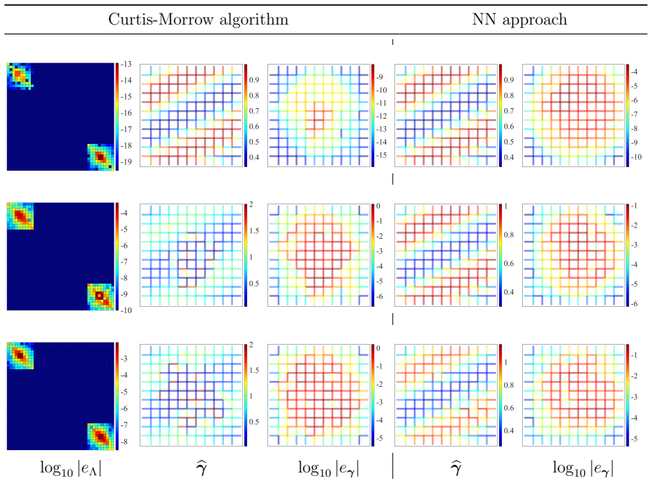
- [Section 5.2.1; Figs. 3-5] The numerical comparison in Section 5, including the abstract's claim that the method outperforms Curtis-Morrow for noisy data, is conditional on the Adam optimizer reaching a zero-loss global minimizer of the nonconvex loss Cα. The paper provides no convergence guarantee, and Section 5.2.1 itself reports that the loss stagnates at positive values for noisy data and that the method fails to give accurate reconstructions for n=20. Theorem 4.1 only characterizes minimizers after they are attained. To make the numerical claims load-bearing, the authors should report the distribution of final loss values and success rates over random initializations, and either prove or clearly state as an assumption the global convergence of the training procedure; in the present form, the comparison tests the optimizer together with the recovery architecture, not the recovery map characterized by Theorem 4.1.
minor comments (5)
- [Notation in Sections 2-3] The paper uses D both for the interior grid in (2.1) and for the full set including ∂D in the architecture discussion; for example, (3.4) indexes outputs by r∈D even though the boundary nodes ∂D are included. Please introduce a separate symbol, e.g., \bar D, and use it consistently throughout.
- [Eq. (4.1)] Weights are indexed by ordered pairs (p,q) although B is a set of unordered edges; specify an orientation convention so that expressions like ew(2)_{pq} and the condition (p,q)∈B are unambiguous.
- [Theorem 6.2] The statement ∇εγ_{T′ε}|_{ε=0}=S†_{T′} should be spelled out as the Jacobian of γ_{T′ε} with respect to the noise vector restricted to T′; as written, the left-hand side has size 2n(n+1)×|T′|, matching the matrix S†_{T′}, but this is not immediately clear from the notation.
- [Abstract and Section 6] The abstract contains the typo 'post-trainig', and Section 6 appears to contain a dimension typo 'R2n(2n+1)' for the conductivity vector, which should be R^{2n(n+1)}.
- [Lemma 6.1] The proof of local smoothness of the extension map is only a sketch; please state the base case of the induction and explicitly note that invertibility of each B_Qk is an open condition that persists in a sufficiently small neighborhood.
Circularity Check
No significant circularity: the weight-recovery theorem is anchored in an external uniqueness theorem and the loss is not constructed from the target conductivities.
full rationale
I find no circular step in the paper's derivation chain. The central claim (Theorem 4.1) is that any zero-loss global minimizer of the mean-square loss (3.6) has second-layer weights equal to the true edge conductivities (up to the paper's stated sign convention). This claim is not self-definitional: the weights ew(2) are unknown optimization variables, and the loss is defined from the DtN data pairs (u(k), v(k)) plus a forward-propagation equation (3.5), not from the target conductivity vector. The proof reduces the zero-loss conditions to the discrete conductivity equations (4.2)/(4.4), which are exactly the physical equations (2.3)-(2.5) with ew(2) playing the role of the conductivity; uniqueness then comes from the external Curtis-Morrow theorem [23, Theorem 5.1], which is a prior mathematical result by different authors, not a self-citation. Thus the uniqueness step is not 'imported from authors' in the sense of this review. The sensitivity formula ∇εγ = S† in Theorem 6.2 is derived from first-order optimality and the Jacobian identity (6.5), not by fitting the error to the sensitivity; it is an independent perturbation calculation. The paper does contain two non-circular weaknesses worth separating from circularity: (i) the numerical success rests on the unproven assumption that Adam reaches a zero-loss global minimizer, which the paper itself notes fails for n = 20 in Section 5.2.1; and (ii) as printed, there appears to be a sign inconsistency between (2.5), (3.4), and (4.1) for boundary edges, so the constructive existence part of Theorem 4.1 may not hold exactly with the displayed weights. Both are correctness or robustness issues, not instances of a claim being equivalent by construction to its inputs. Accordingly, the appropriate circularity score is 0.
Assumptions & free parameters
free parameters (4)
- alpha (loss weighting) =
alpha = 1 in experiments; alpha = infinity in sensitivity analysis
- Adam initial step size =
0.002
- Adam moment decay rates =
first in {0.9, 0.99, 0.999}, second in {0.999, 0.9999}
- random initialization of conductivity =
sampled from R^{2n(n+1)}_+
assumptions (4)
- standard math Curtis-Morrow uniqueness: the DtN matrix, or equivalently the last 3n columns, uniquely determines the edge conductivities on the square lattice.
- standard math The Jacobian of the DtN map with respect to conductivities has full column rank.
- standard math Unique solvability of the discrete Dirichlet problem for any conductivity profile.
- ad hoc to paper The Adam optimizer converges to a global minimizer of the non-convex loss from random initialization.
Cite this review
Pith. "Pith review of The discrete inverse conductivity problem solved by the weights of an interpretable neural network." pith.science (2026). https://pith.science/paper/7WZFM4IR
@misc{pith2026250100345,
  author       = {Pith},
  title        = {Pith review of: The discrete inverse conductivity problem solved by the weights of an interpretable neural network},
  year         = {2026},
  howpublished = {\url{https://pith.science/paper/7WZFM4IR}},
  note         = {Machine review of arXiv:2501.00345}
}
read the original abstract
In this work, we develop a novel neural network (NN) approach to solve the discrete inverse conductivity problem of recovering the conductivity profile on network edges from the discrete Dirichlet-to-Neumann map on a square lattice. The novelty of the approach lies in the fact that the sought-after conductivity is not provided directly as the output of the NN but is instead encoded in the weights of the post-trainig NN in the second layer. Hence the weights of the trained NN acquire a clear physical meaning, which contrasts with most existing neural network approaches, where the weights are typically not interpretable. This work represents a step toward designing NNs with interpretable post-training weights. Numerically, we observe that the method outperforms the conventional Curtis-Morrow algorithm for both noisy full and partial data.
Figures


Figures from the paper (9 more)




Reference graph
Works this paper leans on
-
[1]
N. Akhtar. A survey of explainable ai in deep visual modeling: Methods and metrics. Preprint, arXiv:2301.13445, 2023
work page Pith review arXiv 2023
-
[2]
A. F. Al-Mudhaf. A feed forward neural network approach for matrix computations . PhD thesis, Brunel University, London, 2001. Available at https://bura.brunel. ac.uk/handle/2438/5010. 27
work page 2001
-
[3]
G. Alessandrini. Stable determination of conductivity by boundary measurements. Appl. Anal., 27(1-3):153–172, 1988
work page 1988
-
[4]
G. Alessandrini. Determining conductivity by boundary measurements, the stability issue. In Applied and Industrial Mathematics (Venice, 1989) , volume 56 of Math. Appl., pages 317–324. Kluwer Acad. Publ., Dordrecht, 1991
work page 1989
-
[5]
G. Alessandrini and S. Vessella. Lipschitz stability for the inverse conductivity prob- lem. Adv. Appl. Math. , 35(2):207–241, 2005
work page 2005
-
[6]
D. Alvarez Melis and T. Jaakkola. Towards robust interpretability with self- explaining neural networks. In Advances in Neural Information Processing Systems , volume 31, pages 7786–7795, 2018
work page 2018
-
[7]
E. Beretta and E. Francini. Lipschitz stability for the electrical impedance tomogra- phy problem: the complex case. Comm. Partial Differential Equations , 36(10):1723– 1749, 2011
work page 2011
-
[8]
E. Beretta, S. Micheletti, S. Perotto, and M. Santacesaria. Reconstruction of a piecewise constant conductivity on a polygonal partition via shape optimization in EIT. J. Comput. Phys. , 353:264–280, 2018
work page 2018
Show all 45 references
-
[9]
C. M. Bishop. Neural networks and their applications. Rev. Sci. Instrum., 65(6):1803– 1832, 1994
1994
-
[10]
Bl ˚ asten, H
E. Bl ˚ asten, H. Isozaki, M. Lassas, and J. Lu. Inverse problems for discrete heat equations and random walks for a class of graphs.SIAM J. Discrete Math., 37(2):831– 863, 2023
2023
-
[11]
P. J. Blazek and M. M. Lin. Explainable neural networks that simulate reasoning. Nature Comput. Sci. , 1(9):607–618, 2021
2021
-
[12]
L. Borcea. Electrical impedance tomography. Inverse Problems , 18(6):R99–R136, 2002
2002
-
[13]
Borcea, V
L. Borcea, V. Druskin, and A. V. Mamonov. Circular resistor networks for electri- cal impedance tomography with partial boundary measurements. Inverse Problems, 26(4):045010, 30, 2010
2010
-
[14]
Borcea, V
L. Borcea, V. Druskin, A. V. Mamonov, and F. Guevara Vasquez. Pyramidal resistor networks for electrical impedance tomography with partial boundary measurements. Inverse Problems, 26(10):105009, 36, 2010
2010
-
[15]
Borcea, V
L. Borcea, V. Druskin, and F. G. Vasquez. Electrical impedance tomography with resistor networks. Inverse Problems, 24(3):035013, 2008. 28
2008
-
[16]
Borcea, F
L. Borcea, F. Guevara Vasquez, and A. V. Mamonov. Study of noise effects in electrical impedance tomography with resistor networks. Inverse Probl. Imaging , 7(2):417–443, 2013
2013
-
[17]
Boyer, J
J. Boyer, J. J. Garzella, and F. Guevara Vasquez. On the solvability of the discrete conductivity and Schr¨ odinger inverse problems. SIAM J. Appl. Math. , 76(3):1053– 1075, 2016
2016
-
[18]
S. Cen, B. Jin, K. Shin, and Z. Zhou. Electrical impedance tomography with deep Calder´ on method.J. Comput. Phys. , 493:112427, 2023
2023
-
[19]
Chakraborty
M. Chakraborty. Explainable neural networks: achieving interpretability in neural models. Arch. Comput. Methods Eng. , 31:3535–3550, 2024
2024
-
[20]
F. J. Chung, A. C. Gilbert, J. G. Hoskins, and J. C. Schotland. Optical tomography on graphs. Inverse Problems, 33(5):055016, 21, 2017
2017
-
[21]
Curtis, E
E. Curtis, E. Mooers, and J. Morrow. Finding the conductors in circular networks from boundary measurements. RAIRO Mod´ el. Math. Anal. Num´ er., 28(7):781–814, 1994
1994
-
[22]
E. B. Curtis and J. A. Morrow. Determining the resistors in a network. SIAM J. Appl. Math. , 50(3):918–930, 1990
1990
-
[23]
E. B. Curtis and J. A. Morrow. The Dirichlet to Neumann map for a resistor network. SIAM J. Appl. Math. , 51(4):1011–1029, 1991
1991
-
[24]
Fan and L
Y. Fan and L. Ying. Solving electrical impedance tomography with deep learning. J. Comput. Phys. , 404:109–119, 2020
2020
-
[25]
Gao and L
L. Gao and L. Guan. Interpretability of machine learning: recent advances and future prospects. IEEE MultiMedia, 30(4):105–118, 2023
2023
-
[26]
Garde and K
H. Garde and K. Knudsen. Distinguishability revisited: depth dependent bounds on reconstruction quality in electrical impedance tomography. SIAM J. Appl. Math. , 77(2):697–720, 2017
2017
-
[27]
Guo and J
R. Guo and J. Jiang. Construct deep neural networks based on direct sampling meth- ods for solving electrical impedance tomography. SIAM J. Sci. Comput., 43(3):B678– B711, 2021
2021
-
[28]
S. J. Hamilton and A. Hauptmann. Deep d-bar: real-time electrical impedance to- mography imaging with deep neural networks.IEEE Trans. Med. Imag., 37(10):2367– 2377, 2018. 29
2018
-
[29]
S. Han, J. Pool, J. Tran, and W. Dally. Learning both weights and connections for efficient neural network. In Advances in Neural Information Processing Systems , volume 28, pages 1135–1143, 2015
2015
-
[30]
D. V. Ingerman. Discrete and continuous Dirichlet-to-Neumann maps in the layered case. SIAM J. Math. Anal. , 31(6):1214–1234, 2000
2000
-
[31]
B. Jin, X. Li, Q. Quan, and Z. Zhou. Conductivity imaging from internal mea- surements with mixed least-squares deep neural networks. SIAM J. Imaging Sci. , 17(1):147–187, 2024
2024
-
[32]
D. P. Kingma and J. Ba. Adam: A method for stochastic optimization. In 3rd Inter- national Conference for Learning Representations , San Diego, 2015
2015
-
[33]
Lam and P
T. Lam and P. Pylyavskyy. Inverse problem in cylindrical electrical networks. SIAM J. Appl. Math. , 72(3):767–788, 2012
2012
-
[34]
Li and J
L. Li and J. Hu. An efficient second-order neural network model for computing the Moore–Penrose inverse of matrices. IET Signal Proc. , 16(9):1106–1117, 2022
2022
-
[35]
X. Li, Y. Zhou, J. Wang, Q. Wang, Y. Lu, X. Duan, Y. Sun, J. Zhang, and Z. Liu. A novel deep neural network method for electrical impedance tomography. Trans. Inst. Measure. Control, 41(14):4035–4049, 2019
2019
-
[36]
Mandache
N. Mandache. Exponential instability in an inverse problem for the Schr¨ odinger equation. Inverse Problems, 17(5):1435–1444, 2001
2001
-
[37]
Ronneberger, P
O. Ronneberger, P. Fischer, and T. Brox. U-net: Convolutional networks for biomed- ical image segmentation. In Proceedings of the Eighteenth Conference on Medical Im- age Computing and Computer-Assisted Intervention , pages 234–241. MICCAI, 2015
2015
-
[38]
C. Rudin. Stop explaining black box machine learning models for high stakes decisions and use interpretable models instead. Nature Mach. Intell. , 1(5):206–215, 2019
2019
-
[39]
Rudin, C
C. Rudin, C. Chen, Z. Chen, H. Huang, L. Semenova, and C. Zhong. Interpretable machine learning: Fundamental principles and 10 grand challenges. Stat. Surv. , 16:1–85, 2022
2022
-
[40]
T. J. Sejnowski. The unreasonable effectiveness of deep learning in artificial intelli- gence. Proc. Nat. Acad. Sci. , 117(48):30033–30038, 2020
2020
-
[41]
J. K. Seo, K. C. Kim, A. Jargal, K. Lee, and B. Harrach. A learning-based method for solving ill-posed nonlinear inverse problems: A simulation study of lung EIT. SIAM J. Imaging Sci. , 12(3):1275–1295, 2019. 30
2019
-
[42]
D. N. Tanyu, J. Ning, A. Hauptmann, B. Jin, and P. Maass. Electrical impedance to- mography: A fair comparative study on deep learning and analytic-based approaches. In T. Bubba, editor, Data-Driven Models in Inverse Problems , pages 437–470. de Gruyter, Berlin, 2024
2024
-
[43]
Wang and J
L. Wang and J. M. Mendel. Structured trainable networks for matrix algebra. In International Joint Conference on Neural Networks , pages 125–132, San Diego, CA, 1990
1990
-
[44]
Yuan and Y
M. Yuan and Y. Lin. Model selection and estimation in regression with grouped variables. J. R. Stat. Soc. Ser. B Stat. Method. , 68(1):49–67, 2006
2006
-
[45]
Zhang, P
Y. Zhang, P. Ti˜ no, A. Leonardis, and K. Tang. A survey on neural network inter- pretability. IEEE Trans. Emerg. Topics Comput. Intell. , 5(5):726–742, 2021. 31
2021
Reviewed August 10, 2026 · model on record in the stance chip above.
Discussion (0). Continue with ORCID to comment.