REVIEW 4 major objections 7 minor 31 references
Tensor-structured PCG for finite difference solver of domain patterns in ferroelectric material
T0 review · 4 major / 7 minor · reviewed 2026-08-10 · deepseek-v4-flash
Pith's one-line read A pseudoinverse preconditioner built from the Kronecker structure of the finite-difference Laplacian lets PCG solve cuboid-grid Poisson problems in about two or three iterations.
desk verdict A sound, honest case study whose central speed claim is plausible but not demonstrated by the reported experiments. read the letter →
The pith
A machine-rendered reading of the paper's core claim, the machinery that carries it, and where it could break.
The reading
What carries the argument
The load-bearing object is the family of 1D finite-difference Laplacians $L_n(\alpha,\beta,\gamma)$, whose four boundary-condition variants (periodic, Dirichlet, Neumann, mixed) have closed-form sine-and-cosine eigen-decompositions (Lemmas 3.1-3.4). The 2D/3D discrete Laplacian is the Kronecker sum of these 1D matrices, so its eigenvalues are sums of 1D eigenvalues and its eigenvectors are Kronecker products of 1D eigenvectors. The Moore-Penrose pseudoinverse preconditioner $M_{\mathrm{p-inv}}$ exploits this by applying $V_n^T R V_q$, multiplying entrywise by the Hadamard pseudoinverse of the matrix of eigenvalue sums $(\lambda_i+\lambda_j)^{\dagger}$, and transforming back with $V_n F V_q^T$ (Algorithms 4-7), which the paper identifies as a Fourier-solver step for the residual.
What would settle it
Take a dense, null-space-orthogonal right-hand side on a cuboid grid with periodic boundary conditions in all directions and run PCG with the pseudoinverse preconditioner; if the true residual has not dropped to near machine precision relative to the initial residual within three iterations (the paper's stated 'two or three are sufficient'), the central convergence claim is refuted. A concrete target: on the $512\times 256\times 8$ problem described in Section 5, count iterations to reach $\|H-\mathcal{L}U_s\|_F/\|H\|_F \le 10^{-10}$ and check whether the count is at most three.
Extended reading notes
Core claim
The central discovery is that the Moore-Penrose pseudoinverse of the Kronecker-structured finite-difference Laplacian is an almost perfect preconditioner for PCG on this problem. Writing the 2D operator as $(I_q\otimes L_n)+(L_q\otimes I_n)$, the eigenvectors are Kronecker products of the 1D Laplacian eigenvectors and the eigenvalues are sums $\lambda_i(L_n)+\lambda_j(L_q)$; the pseudoinverse preconditioner transforms the residual into this eigenbasis, divides by the nonzero eigenvalue sums (treating sums below $10^{-13}$ as zero), and transforms back. In the authors' experiments the true residual is essentially at the desired level after the first iteration and fully converged after two or three, so the paper proposes viewing the scheme as a pseudoinverse-based direct solver with refinement by CG iteration. The same construction extends to 3D with a three-way tensor and triples of eigenvalue sums.
Load-bearing premise
The claim rests on being able to store and multiply dense $n\times q$ (or $n\times q\times t$) arrays, because the right-hand side and all intermediate objects in the preconditioner are dense; if only sparse matrix storage fits in memory, this preconditioner's advantage over sparse iterative solvers disappears.
Editorial extensions
If this is right
- For the simple Laplace operator on a cuboid, PCG with the pseudoinverse preconditioner needs only two or three iterations to converge; the authors run ten to be safe.
- The method behaves as a direct solver: the pseudoinverse application produces an almost-exact solution and the CG outer loop removes the residual left by the eigenvalue-sum threshold.
- The per-iteration cost is $O(nq(n+q))$ in 2D and $O(nqt(n+q+t))$ in 3D, comparable to the unpreconditioned PCG iteration itself, with initialization cost dominated by the eigendecompositions of the 1D Laplacians.
- For singular Laplacians (periodic or Neumann in all directions), centering the data and thresholding the pseudoinverse keeps the iteration in the null-space-orthogonal subspace, so the solution is recovered up to the expected additive constant.
- The approach has been implemented in C/C++ and used to produce published results on ferroelectric domain walls cited in the paper.
Reading between the lines
- Because the pseudoinverse preconditioner is a trigonometric (Fourier-type) solver, on strongly anisotropic grids where one dimension is much smaller than the others the per-iteration cost $O(nqt(n+q+t))$ can exceed that of an FFT-based Poisson solver with $O(N\log N)$ work; the paper's method is best suited to near-cubic grids where the dense-array storage is already affordable.
- The same pseudoinverse-of-the-Kronecker-sum construction should transfer to other separable operators on cuboids, for example anisotropic diffusion with different coefficients per axis or Schrodinger operators with separable potentials, whenever the 1D factors have known eigendecompositions; the paper's experiments only cover the scalar homogeneous Laplacian.
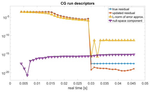
- The $10^{-13}$ threshold means the method is not a true direct solver for systems with very small nonzero eigenvalues; the number of CG iterations would grow if the right-hand side had significant energy in near-null directions, so one could probe robustness by constructing such right-hand sides explicitly.
Signed reviews
Editorial analysis
A structured set of objections, weighed in public.
Referee Report
Summary. The paper studies the preconditioned conjugate gradient (PCG) solution of finite-difference discretizations of Poisson's equation on rectangular or cuboid domains, where the discrete Laplacian is a sum of Kronecker products. The authors derive three preconditioners adapted to this structure: a Jacobi-like fixed-point preconditioner, a low-Kronecker-rank approximate inverse, and a Moore-Penrose pseudoinverse of the discretized Laplacian. The pseudoinverse preconditioner is built from analytic spectral decompositions of the one-dimensional Laplacians and is applied through basis transformations and Hadamard multiplication. Numerical experiments on six 2D and three 3D right-hand sides show rapid residual decrease, and the paper concludes that two or three PCG iterations are sufficient for this problem.
Significance. The mathematical derivation of the pseudoinverse preconditioner from the eigendecompositions of the 1D Laplacians is correct and standard, and the paper honestly identifies the method as a pseudoinverse-based direct solver with CG refinement. If the performance claims are substantiated, the method is a practical and simple Fourier-like preconditioner for Kronecker-structured Poisson problems with dense right-hand sides, and the connection to the Ferrodo2 application in ferroelectric simulation is valuable. The paper also provides explicit algorithms, analytical eigenvector formulas, and cost tables, which are useful for reproduction. However, the central efficiency claim is currently supported mainly by wall-clock plots with post hoc iteration counts and no comparison against standard baselines, so the significance of the numerical evidence is not yet at the level of the paper's conclusions.
major comments (4)
- [§5.2, Remark 4.2, Fig. 9] The central claim in Section 6 that two or three PCG iterations are sufficient is not supported by the reported data. Remark 4.2 states that the iteration number is fixed experimentally so that the true residual decreases sufficiently, but no target residual or achieved residual is reported. Section 5.2 selects iteration counts post hoc, and Figure 9 shows only wall-clock time after initialization, with no iteration counts for any of the nine test cases. Since the pseudoinverse preconditioner is the exact inverse on the range of the operator, one iteration is expected in exact arithmetic; the practical question is how many iterations are needed in floating-point arithmetic at a specified relative tolerance. The paper does not answer this question, and the claim is therefore not reproducible from the presented data. Please provide a table of iteration counts and true residual norms relative to the normalized initial residual for each test problem.
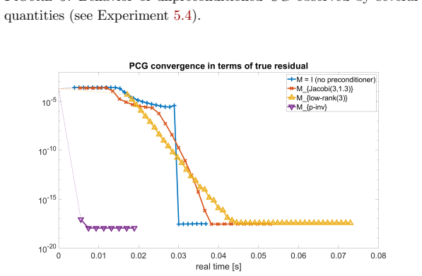
- [§5.2, Figs. 4–9] The performance comparison lacks essential baselines. Figure 6 compares preconditioners only on a single 50×100 problem, and the larger 2D and 3D runs in Figure 9 report only pseudoinverse-preconditioned PCG times. No comparison is made with unpreconditioned sparse CG, a sparse direct solver, or an FFT-based direct solver, even though Remark 4.3 identifies the pseudoinverse preconditioner as essentially a Fourier solver. Without such baselines, the conclusion that the method is extremely efficient for practical problem sizes is not established. Please report timings, iteration counts, and achieved residuals against at least one standard sparse solver and one FFT/direct solver for the nine test problems.
- [§5.2, Eq. (5.1)] The residual metric used in the experiments is not adequate for the application claim. Equation (5.1) normalizes the initial residual norm to 1/(nq) or 1/(nqt), so plots of absolute residual norms are not comparable across grids, and no relative tolerance is specified. In addition, the physically relevant output for the ferroelectric application is the electric field, i.e., the gradient of the potential, but the paper reports only residual norms and does not report error in the gradient. Please report relative residual norms and, where possible, the error in the computed electric field relative to a reference solution.
- [§6] The applicability of the method depends critically on the ability to store dense right-hand sides and dense intermediate matrices of size O(nq) or O(nqt). Section 6 acknowledges this, but the limitation should be stated more prominently, and the numerical experiments should include a memory comparison with sparse iterative solvers for the reported grid sizes. In regimes where dense storage is infeasible, the method loses its claimed advantage; the paper should make the scope of the efficiency claim explicit and quantify at which grid sizes the dense approach becomes impractical.
minor comments (7)
- [Problem 5.2] The phrase 'Newton condition e_R = -1/2' should be 'Neumann condition'.
- [Lemma 3.4] The two formulas for the eigenvectors v_k are not explicitly assigned to L_{n,DN} and L_{n,ND}; please label them clearly.
- [§4.2] The indices ζ and ξ are used for entries of W without being defined; please replace them with i and j or define them in the notation section.
- [§4.1 and Algorithm 1] There are small language issues: 'spaned' should be 'spanned', and 'Until stopping criterion match' should be 'Until stopping criterion matches'.
- [§4.3.2] The paper states that no algorithmic description of the low-Kronecker-rank preconditioner is provided, yet this preconditioner is used in the experiments reported in Figures 6–8. Please either provide the algorithm or describe more precisely how the experiments were implemented, so that the comparison is reproducible.
- [Abstract and Section 1] Please proofread for language issues such as 'preconditioners that fits', 'homogenous', and 'isotropous'.
- [Fig. 9 caption] The caption claims the convergence curve is 'almost problem independent', but the plot uses wall-clock time after initialization on a log scale and shows no iteration counts; please rephrase or provide the actual iteration counts and residual values.
Circularity Check
No significant circularity: the pseudoinverse preconditioner is derived from the operator's own spectral decomposition, and the paper explicitly identifies the result as a direct solver with CG refinement.
full rationale
The derivation chain is self-contained. The pseudoinverse preconditioner is constructed from the analytical eigendecompositions of the one-dimensional finite-difference Laplacians (Lemmas 3.1-3.4), and equations (3.5), (4.5)-(4.7), and Algorithms 4-7 then build L-dagger from those spectra; no output quantity is fed back into the construction. The rapid convergence of PCG with M = L-dagger is a mathematical consequence, not an empirical prediction: on the range of L the preconditioned operator is the identity, so exact arithmetic terminates in essentially one step, and the paper acknowledges this by calling the method 'a pseudoinverse-based direct solver with iterative refinement by CG iteration' (Section 6) and noting it is 'essentially a Fourier solver' (Remark 4.3). The claimed two-to-three iterations are therefore explained by construction, not discovered from fitted data. Self-citations ([15], [16]) are used only as external application context and are not load-bearing for the numerical analysis. The experimental protocol fixes iteration counts to make residuals 'sufficiently' small (Remark 4.2, Section 5.2) and normalizes initial residuals to 1/N, which weakens reproducibility of the few-iteration claim, but this is a reporting limitation, not a circular reduction of the derivation to its inputs.
Assumptions & free parameters
free parameters (4)
- Pseudoinverse eigenvalue threshold =
1e-13
- Jacobi preconditioner parameters (p, omega) =
p=3, omega=1.3
- Low-rank approximation rank rK =
rK=3
- Number of PCG iterations in final experiments =
10
assumptions (5)
- standard math Spectral properties of 1D finite-difference Laplacians Ln(alpha,beta,gamma) stated in Lemmas 3.1-3.4, including eigenvectors for periodic, Dirichlet, Neumann, and mixed BCs.
- standard math Moore-Penrose pseudoinverse properties and the Eckart-Young-Mirsky theorem for low-rank approximation.
- domain assumption The material is homogeneous and isotropic with scalar permittivity, and the domain is a rectangle or cuboid with a regular finite-difference grid.
- domain assumption The right-hand side H is dense with general rank(s), and its size allows storing several dense matrices of O(nq) or O(nqt) entries.
- ad hoc to paper Eigenvalue sums with modulus below 1e-13 are treated as zero when forming the pseudoinverse.
Cite this review
Pith. "Pith review of Tensor-structured PCG for finite difference solver of domain patterns in ferroelectric material." pith.science (2026). https://pith.science/paper/H6QVTGSR
@misc{pith2026250103377,
  author       = {Pith},
  title        = {Pith review of: Tensor-structured PCG for finite difference solver of domain patterns in ferroelectric material},
  year         = {2026},
  howpublished = {\url{https://pith.science/paper/H6QVTGSR}},
  note         = {Machine review of arXiv:2501.03377}
}
read the original abstract
This paper presents a case study of application of the preconditioned method of conjugate gradients (CG) on a problem with operator resembling the structure of sum of Kronecker products. In particular, we are solving the Poisson's equation on a sample of homogeneous isotropic ferroelectric material of cuboid shape, where the Laplacian is discretized by finite difference. We present several preconditioners that fits the Kronecker structure and thus can be efficiently implemented and applied. Preconditioner based on the Moore--Penrose pseudoinverse is extremely efficient for this particular problem, and also applicable (if we are able to store the dense right-hand side of our problem). We briefly analyze the computational cost of the method and individual preconditioners, and illustrate effectiveness of the chosen one by numerical experiments. Although we describe our method as preconditioned CG with pseudoinverse-based preconditioner, it can also be seen as pseudoinverse-based direct solver with iterative refinement by CG iteration. This work is motivated by real application, the method was already implemented in C/C++ code Ferrodo2 and first results were published in Physical Review B 107(9) (2023), paper id 094102.
Figures


Figures from the paper (7 more)



Reference graph
Works this paper leans on
-
[1]
A. Ben-Israel, T. N. E. Greville : Generalized Inverses: Theory and Applications (2nd ed.). Springer, New York, 2003. Zbl 1026.15004, DOI 10.1007/b97366
-
[2]
J. D. Carroll, J. Chang : Analysis of individual differences in multidimensional scaling via an n-way generalization of “Eckart–Young” decomposition, Psychometrika. 35 (3) (1970), pp. 283–319. Zbl 0202.19101, DOI 10.1007/BF02310791
- [3]
-
[4]
L. C. Evans : Partial differential equations (2nd ed.), Graduate Studies in Mathemat- ics Volume 19, American Mathematical Society, Providence, 2010. Zbl 1194.35001, DOI 10.1090/gsm/019 29 Figure 10. Approximate solutions of all three problems. Vertical axis measures the electric potential (in the bottom plot, there is the vertical scale related to the fi...
arXiv 2010
-
[5]
R. P. Feynman : Feynman lectures on physics. Vol. 2, Mainly electromagnetism and matter, Addison-Wesley, Reading, 1964
work page 1964
-
[6]
M. Fiedler: Special matrices and their applications in numerical mathematics (2nd ed.), Dover Publications, Dover, 2008. Zbl 1170.65018
- [7]
-
[8]
R. A. Harshman, Richard Foundations of the PARAF AC procedure: Models and conditions for an “explanatory” multi-modal factor analysis, UCLA Working Papers in Phonetics 16, 1970
work page 1970
Show all 31 references
-
[9]
M. R. Hestenes, E. Stiefel : Methods of conjugate gradients for solving linear systems, Journal of Research of the National Bureau of Standards 49(6) (1952), pp. 409–436. Zbl 0048.09901, DOI 10.6028/jres.049.044
1952
-
[10]
Kol´ arov´ a: Spectral properties of discretized Laplace operator (in Czech), Diploma the- sis, Technical University of Liberec, 2024
J. Kol´ arov´ a: Spectral properties of discretized Laplace operator (in Czech), Diploma the- sis, Technical University of Liberec, 2024. URL https://stag.tul.cz/StagPortletsJSR168/ CleanUrl?urlid=prohlizeni-prace-detail&praceIdno=47663
2024
-
[11]
T. G. Kolda, B. W. Bader : Tensor decompositions and applications, SIAM Review 51(3) (2009), pp. 455–500. Zbl 1173.65029, DOI 10.1137/07070111X
2009
-
[12]
Kressner, M
D. Kressner, M. Pleˇ singer, C. Tobler, A preconditioned low-rank CG method for parameter- dependent Lyapunov matrix equations, Numerical Linear Algebra with Applications 21(5) (2014), pp. 666–684. Zbl 1340.65077, DOI 10.1002/nla.1919
2014
-
[13]
Liesen, Z
J. Liesen, Z. Strakoˇ s: Krylov subspace methods: Principles and analysis, Oxford University Press, Oxford, 2012. Zbl 1307.65001, DOI 10.1093/acprof:oso/9780199655410.001.0001
2012
-
[14]
M´ alek, Z
J. M´ alek, Z. Strakoˇ s: Preconditioning and the conjugate gradient method in the con- text of solving PDEs, SIAM Spotlights 1, Phildelphia, 2015. Zbl 1396.65002, DOI 10.1137/1.9781611973846
2015
-
[15]
Marton, M
P. Marton, M. A. P. Gon¸ calves, M. Pa´ sciak, S. K¨ orbel, V. Chumchal, M. Pleˇ singer, A. Kl ´ ıˇ c, J. Hlinka : Zigzag charged domain walls in ferroelectric PbTiO 3, Physical Review B 107(9) (2023), paper id 094102, pp. 1–9. DOI 10.1103/PhysRevB.107.094102
2023 doi
-
[16]
Marton, J
P. Marton, J. Hlinka : Simulation of domain patterns in BaTiO 3, Phase Transitions 79(6–7) (2006), pp. 467–483. DOI 10.1080/01411590600892351
2006 doi
-
[17]
J. C. Maxwell : A dynamical theory of the electromagnetic field, Philosophical Transactions of the Royal Society of London 155 (1865), pp. 459–512. DOI 10.1098/rstl.1865.0008
-
[18]
Meurant : The Lanczos and conjugate gradient algorithms: From theory to finite pre- cision computations, SIAM Software, Environments, and Tools 19, Philadelphia, 2006
G. Meurant : The Lanczos and conjugate gradient algorithms: From theory to finite pre- cision computations, SIAM Software, Environments, and Tools 19, Philadelphia, 2006. Zbl 1110.65029, DOI 10.1137/1.9780898718140
2006
-
[19]
Meurant, J
G. Meurant, J. Papeˇ z, P. Tich´ y: Accurate error estimation in CG, Numerical Algorithms 88(3) (2021), pp. 1337–1359. Zbl 1490.65056, DOI 10.1007/s11075-021-01078-w
2021
-
[20]
Meurant, P
G. Meurant, P. Tich´ y: Error norm estimation in the conjugate gradient algorithm, SIAM Spotlights 6, Phildelphia, 2024. Zbl 07851831, DOI 10.1137/1.9781611977868
2024 doi
-
[21]
Mirsky : Symmetric gauge functions and unitarily invariant norms, The Quarterly Jour- nal of Mathematics, Oxford Second Series, 11 (1960), pp
L. Mirsky : Symmetric gauge functions and unitarily invariant norms, The Quarterly Jour- nal of Mathematics, Oxford Second Series, 11 (1960), pp. 50–59. Zbl 0105.01101, DOI 10.1093/qmath/11.1.50
1960
-
[22]
B. N. Parlett : The symmetric eigenvalue problem (unabridged, corrected republication of 1980), SIAM Classics in Applied Mathematics 20, Phildelphia, 1998. Zbl 0885.65039, DOI 10.1137/1.9781611971163
1980
-
[23]
Saad : Numerical methods for large eigenvalue problems (revised ed.) SIAM Classics in Applied Mathematics 66, Phildelphia, 2011
Y. Saad : Numerical methods for large eigenvalue problems (revised ed.) SIAM Classics in Applied Mathematics 66, Phildelphia, 2011. Zbl 1242.65068, DOI 10.1137/1.9781611970739
2011
-
[24]
L. R. Tucker: Implications of factor analysis of three-way matrices for measurement of change, Problems in Measuring Change (C. W. Harries ed.), University of Wisconsin Press, Madison, WI, 1963, pp. 122–137
1963
-
[25]
L. R. Tucker : The extension of factor analysis to three-dimensional matrices, in: Contribu- tions to Mathematical Psychology (H. Gulliksen and N. HoltFrederiksen eds.), Holt, Rinehardt & Winston, New York, 1964, pp. 110–127. 31
1964
-
[26]
L. R. Tucker : Some mathematical notes on three-mode factor analysis, Psychometrika, 31 (1966), pp. 279–311, DOI 10.1007/BF02289464
1966 doi
-
[27]
D. A. Turkington: Generalized vectorization, cross-products, and matrix calculus, Cambridge University Press, Cambridge, 2013. Zbl 1307.15001, DOI 10.1017/CBO9781139424400
2013
-
[28]
Ullmann : A Kronecker product preconditioner for stochastic Galerkin finite element dis- cretization, SIAM Journal on Scientific Computing, 32 (2010), pp
E. Ullmann : A Kronecker product preconditioner for stochastic Galerkin finite element dis- cretization, SIAM Journal on Scientific Computing, 32 (2010), pp. 923–946. Zbl 1210.35306, DOI 10.1137/080742853
2010
-
[29]
R. S. Varga: Matrix iterative analysis (2nd revised and expanded ed.), Springer, Berlin, 2000. Zbl 0998.65505, DOI 10.1007/978-3-642-05156-2
2000
-
[30]
E. Wang, Q. Zhang, B. Shen, G. Zhang, X. Lu, Q. Wu, Y. Wang : Intel Math Kernel Library, in: High-Performance Computing on the Intel R○ Xeon Phi™, Springer, Cham, 2014, pp. 167–188. DOI 10.1007/978-3-319-06486-4 7
2014 doi
-
[31]
URL https://www.intel.com/content/www/ us/en/developer/tools/oneapi/onemkl.html
Intel R○ oneAPI Math Kernel Library (oneMKL). URL https://www.intel.com/content/www/ us/en/developer/tools/oneapi/onemkl.html. Authors’ addresses : Vˇ enceslav Chumchal, Department of Mathematics, Technical University of Liberec, Studentsk´ a 1402/2, 461 17 Liberec 1, Czech Re...
Reviewed August 10, 2026 · model on record in the stance chip above.
Discussion (0). Continue with ORCID to comment.