REVIEW 3 major objections 5 minor 41 references
Monthly GDP Growth Estimates for the U.S. States
T0 review · 3 major / 5 minor · reviewed 2026-08-10 · deepseek-v4-flash
Pith's one-line read Monthly GDP for every U.S. state can be estimated directly from official annual and quarterly data, and nowcast months before the official release, using one jointly estimated Bayesian model.
desk verdict A genuinely useful measurement paper whose pre-2005 historical series rests on an unvalidated MCMC shortcut; referees should ask for a small-scale exact-MCMC check and a clearer statement of the lead-time claims. read the letter →
The pith
A machine-rendered reading of the paper's core claim, the machinery that carries it, and where it could break.
The reading
What carries the argument
The central object is a mixed-frequency vector autoregression written as a state-space model whose latent states are monthly values of variables observed only quarterly or annually, plus a cross-sectional adding-up restriction. Temporal consistency is enforced by exact aggregation identities: quarterly growth is a weighted average of five adjacent monthly growth rates, and annual growth a weighted average of 23 adjacent monthly rates. Cross-sectional consistency is enforced by a separate measurement equation that makes state GDP sum to U.S. GDP, with a small estimated error. The horseshoe prior shrinks the many VAR coefficients equation by equation, and the approximate MCMC algorithm splits the three-way annual–quarterly–monthly mismatch into two two-way blocks, avoiding the computationally heavy annual–monthly restriction while still conditioning the monthly draws on monthly data.
What would settle it
Run the exact, non-approximate estimation routine on a three-state version of the same model over a pre-2005 subsample, for example 1990 through 2004, and compare its posterior draws of monthly state GDP growth with those from the approximate two-block algorithm; if the credible intervals for the differences exclude zero, the approximation is not negligible and the historical monthly series is compromised.
Extended reading notes
Core claim
The central claim is that state-level GDP can be estimated and nowcast at monthly frequency with one large mixed-frequency VAR in which the unobserved monthly state series is the object of interest. The model writes each state's monthly GDP as part of a state-space system where quarterly and annual observations enter through a weighted temporal aggregation rule, and where state GDP adds up to U.S. GDP through a cross-sectional restriction with a stochastic error that absorbs the overseas accounting wedge and vintage differences. Estimation is joint across all 51 units, so shocks can spill across states and the more timely U.S. GDP releases can be apportioned among states rather than ignored. The paper reports that this joint constrained model produces historical monthly estimates that align with official data at the observed low frequencies, and that in real-time evaluation from 2007 to 2024 its nowcasts are more accurate than those from a benchmark that neither allows cross-state dependencies nor imposes the cross-sectional constraint, with the largest improvement appearing at the third month of the quarter.
Load-bearing premise
The load-bearing assumption is that, for the pre-2005 sample, replacing the monthly U.S. indicators with their quarterly averages in one step of the estimation discards almost no information; if that loss is not small, the historical monthly state GDP series is biased in a way the paper does not measure.
Editorial extensions
If this is right
- State-level business cycles can be dated at monthly frequency from 1964 onward: the paper's median estimates imply Florida and Georgia saw three recessions since 1964, while Iowa, North Dakota, and Alaska saw thirteen or fourteen.
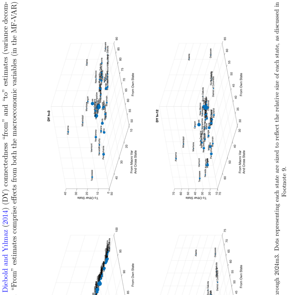
- Cross-state spillovers can be measured at a monthly horizon: the paper's variance-decomposition analysis shows many states shift from mostly own-state shocks to strong macro and cross-state spillovers within three months of a shock.
- Real-time nowcasts made at the end of the third month of a quarter are accurate enough to replace waiting for the official state release, and the biggest accuracy gain arrives when U.S. GDP for that quarter becomes known.
- A joint model with the cross-sectional constraint beats a state-by-state mixed-frequency VAR on average RMSE and CRPS from the third month onward, so conditioning on U.S. GDP and other states' data is doing real work.
- The monthly historical series and updated nowcasts are maintained and posted online, so the estimates are intended as a continuing product for regional analysis rather than a one-off exercise.
Reading between the lines
- An extension left implicit is that the same two-block approximation should carry over to any panel with a changing frequency mismatch, so the computational device is not tied to U.S. states; a regional output panel in another country with annual-then-quarterly data could reuse it directly.
- A natural decomposition experiment would run the out-of-sample exercise four ways—with and without cross-state VAR dynamics, and with and without the cross-sectional constraint—to quantify how much of the third-month gain comes from each ingredient; the paper only compares the full model against the fully restricted benchmark.
- Because the cross-sectional weights are held at fixed annual shares, a testable refinement is to let them vary each year or quarter; states with trending output shares would be the place to look for differences, even though the paper reports the fixed-weight choice is not driving its results.
- The paper notes weekly estimates are possible but costly; a weekly extension would matter most for pandemic-period tracking, where intra-month movements were large, and the model's latent-state structure is already a natural fit for that higher frequency.
Editorial analysis
A structured set of objections, weighed in public.
Referee Report
Summary. This paper develops a large Bayesian mixed-frequency vector autoregression (MF-VAR) that produces monthly real GDP estimates for the 50 U.S. states plus Washington, DC, from 1964 to 2024, using monthly U.S. indicators, quarterly U.S. GDP, quarterly state GDP from 2005, and annual state GDP before 2005. Temporal and cross-sectional aggregation constraints are imposed so that the latent monthly state series aggregates exactly to official BEA quarterly state and U.S. GDP. Estimation is based on a horseshoe-prior shrinkage and an approximate two-block MCMC algorithm that separates an annual/quarterly model from a quarterly/monthly model. The paper reports historical monthly state GDP estimates, business-cycle dating and connectedness analyses, and a real-time nowcasting exercise for 2007Q1-2024Q1 in which the joint model is compared with a state-specific MF-VAR benchmark.
Significance. If the results hold, the paper offers a new and potentially valuable data product: monthly state GDP estimates that are exactly consistent with official BEA aggregates by construction, plus a nowcasting tool with a lead over official releases. The strengths are the exact temporal and cross-sectional constraints, the real-time out-of-sample evaluation against a reasonable benchmark, the use of a horseshoe prior in a high-dimensional MF-VAR, and the transparency about the computational obstacles. The central caveat is that the pre-2005 historical monthly series depends on an unquantified approximation in Section 2.5, so the historical component of the product is not yet validated to the same standard as the post-2007 nowcast results.
major comments (3)
- [Section 2.5, Eq. (8)] The two-block MCMC algorithm conditions the annual/quarterly block on quarterly aggregates of the U.S. monthly variables rather than on the monthly series themselves. The paper's only justification is the sentence 'the loss of information is likely to be small,' and no simulation, sensitivity analysis, or error bound is given. Since draws of quarterly state GDP from this approximate block are then fed into the first factor in Eq. (8) that generates the monthly state GDP series, the approximation propagates into every pre-2005 monthly estimate and into the business-cycle and connectedness results based on those estimates. I request a small-scale exact-MCMC comparison (for example, on a few states with the same data frequencies) or a simulation study demonstrating that posterior medians and credible intervals for state GDP are insensitive to replacing monthly U.S. indicators with their quarterly aggregates.
- [Section 3.3, Tables 1-4] The out-of-sample evaluation covers only 2007Q1-2024Q1 and therefore only the regime in which quarterly state GDP is observed throughout; it does not validate the 1964-2004 historical monthly series that is produced under the annual-only regime and the approximate algorithm. The abstract's nowcast claim concerns the modern regime, but the paper's historical data product is a central output. The authors should either state this limitation prominently and supply the exact-MCMC validation from the previous comment, or provide an additional validation exercise for the annual-only regime (for example, a pseudo-out-of-sample experiment using annual data only).
- [Footnote 9 and Section 3.2.1] The claim that fixing the cross-sectional weights at sample averages and ignoring temporal variation in state GDP shares 'does not affect our results' is asserted without supporting evidence. Since the cross-sectional restriction in Eq. (6) is the main channel through which U.S. GDP information is allocated across states, this sensitivity claim is not self-evident over a sample with large shifts in regional composition; please report the numerical comparison with time-varying weights or qualify the claim.
minor comments (5)
- [Section 3.2.1, Figure 1] The statement in Section 3.2.1 that the model-based estimates 'align' with the BEA estimates at observed dates should be rephrased: this alignment is imposed by the temporal aggregation constraints and therefore cannot be read as evidence of in-sample fit.
- [Section 4, Conclusion] The conclusion says the nowcasts are available 'four month ahead of the BEA's first estimates,' while the abstract says three months and Section 3.3 mentions two- and five-month leads for different horizons; please reconcile the timing claims and fix the singular/plural error.
- [Section 2.3, Eqs. (3)-(5)] Equations (3)-(5) are presented as exact restrictions on 'exact' growth rates, but the standard Mariano-Murasawa linear form is derived for log-differenced variables; please clarify the sense in which these equations are exact for x_t/x_{t-1}-1 and, if they are approximations, quantify the approximation error.
- [Online Appendix A.2, Eqs. (7)-(13)] The state-space notation in Equations (7)-(13) of Appendix A.2 would benefit from a table defining the dimensions of the blocks (N_HF, N_LF, p) and the relationship between the two-step algorithm and the two blocks, to make the implementation reproducible.
- [Section 3.3] The evaluation drops 2020Q2-Q4 because of COVID-19 outliers, but the historical monthly estimates cover the pandemic period; a brief statement of how the smoothed historical estimates are affected by those observations would help readers interpret Figure 1 and the business-cycle results.
Circularity Check
No significant circularity: the paper's BEA consistency is explicitly imposed via aggregation constraints, and its nowcast claims rest on out-of-sample comparisons against BEA data and a restricted benchmark.
full rationale
The derivation chain is not circular. The paper specifies a state-space MF-VAR whose measurement equations (3)-(6) impose temporal and cross-sectional aggregation of latent monthly state GDP to observed quarterly/annual state GDP and to U.S. GDP. The resulting 'consistency' with BEA data is by construction, and the paper says so: 'As expected, given imposition of the temporal aggregation constraints, we see that ... the model-based estimates align with the BEA estimates.' That is an accounting restriction, not a prediction used to validate the model. The substantive claims are tested out-of-sample: recursive nowcasts and estimates are compared with BEA vintages (Tables 1-4) and with a restricted benchmark MF-VAR that omits cross-state links and the cross-sectional constraint; the ratios below unity in Tables 3-4 are empirical findings, not identities. The cross-sectional error variance sigma_cs^2 is given an inverse-gamma prior and estimated (Eq. 7), so it is not fixed to force fit. Citations to Koop et al. (2020b, 2024) supply standard mixed-frequency aggregation identities and an estimation framework; these identities are simple accounting definitions and are not invoked as a uniqueness theorem, so they are not load-bearing self-citations. The approximate MCMC split in Section 2.5 replaces monthly U.S. indicators by quarterly aggregates in one posterior block, justified by an unquantified 'loss of information is likely to be small' claim; this is a stated approximation affecting uncertainty and historical estimates, but it is not a circular reduction because the monthly block p(y^S_{a,m}|y^S_{a,q}, y^{US}_q, y^{US}_m) still conditions on monthly data and the annual data enter through the separate annual/quarterly block. Overall, no step in the derivation reduces by construction to its own inputs.
Assumptions & free parameters
free parameters (2)
- sigma^2_cs =
not reported; estimated from data with IG(10,0.01) prior
- Lag length p =
5
assumptions (5)
- standard math Quarterly and annual growth rates are exact weighted sums of monthly growth rates (Eqs. 3-5, Mariano-Murasawa approximation).
- domain assumption U.S. GDP equals the sum of state GDP plus an error term (Eq. 6).
- domain assumption State output shares w_s,t can be proxied by annual averages with negligible within-year variation.
- ad hoc to paper The approximate two-block MCMC algorithm loses negligible information.
- domain assumption The U.S. GDP deflator is an acceptable deflator for state-level nominal GDP before 1977.
invented entities (1)
-
Latent monthly state-level GDP (y^s_{a,m,t})
independent evidence
Cite this review
Pith. "Pith review of Monthly GDP Growth Estimates for the U.S. States." pith.science (2026). https://pith.science/paper/QE7DOMA4
@misc{pith2026250104607,
  author       = {Pith},
  title        = {Pith review of: Monthly GDP Growth Estimates for the U.S. States},
  year         = {2026},
  howpublished = {\url{https://pith.science/paper/QE7DOMA4}},
  note         = {Machine review of arXiv:2501.04607}
}
read the original abstract
This paper develops a mixed frequency vector autoregressive (MF-VAR) model to produce nowcasts and historical estimates of monthly real state-level GDP for the 50 U.S. states, plus Washington DC, from 1964 through the present day. The MF-VAR model incorporates state and U.S. data at the monthly, quarterly, and annual frequencies. Temporal and cross-sectional constraints are imposed to ensure that the monthly state-level estimates are consistent with official estimates of quarterly GDP at the U.S. and state-levels. We illustrate the utility of the historical estimates in better understanding state business cycles and cross-state dependencies. We show how the model produces accurate nowcasts of state GDP three months ahead of the BEA's quarterly estimates, after conditioning on the latest estimates of U.S. GDP.
Figures



Figures from the paper (1 more)
Reference graph
Works this paper leans on
-
[1]
, " * write output.state after.block = add.period write newline
ENTRY address author booktitle chapter doi edition editor eid howpublished institution journal key month note number organization pages publisher school series title type url volume year label extra.label sort.label short.list INTEGERS output.state before.all mid.sentence after.sentence after.block FUNCTION init.state.consts #0 'before.all := #1 'mid.sent...
-
[2]
" write newline "" before.all 'output.state := FUNCTION if.digit duplicate "0" = swap duplicate "1" = swap duplicate "2" = swap duplicate "3" = swap duplicate "4" = swap duplicate "5" = swap duplicate "6" = swap duplicate "7" = swap duplicate "8" = swap "9" = or or or or or or or or or FUNCTION n.separate 't := "" #0 'numnames := t empty not t #-1 #1 subs...
-
[3]
Simulation smoothing for nowcasting with large mixed-frequency VAR s
Ankargren, Sebastian and Paulina Jonéus (2021). Simulation smoothing for nowcasting with large mixed-frequency VAR s. Econometrics and Statistics, 19, pp. 97--113. doi:10.1016/j.ecosta.2020.05.007
-
[4]
Arias, Maria A., Charles S. Gascon, and David E. Rapach (2016). Metro business cycles. Journal of Urban Economics, 94, pp. 90--108. doi:10.1016/j.jue.2016.05.005
-
[5]
Tracking weekly state-level economic conditions
Baumeister, Christiane, Danilo Leiva-León, and Eric Sims (2024). Tracking weekly state-level economic conditions. The Review of Economics and Statistics, 106(2), pp. 483--504. doi:10.1162/rest_a_01171
-
[6]
Large B ayesian vector auto regressions
Bańbura, Marta, Domenico Giannone, and Lucrezia Reichlin (2010). Large B ayesian vector auto regressions. Journal of Applied Econometrics, 25(1), pp. 71--92. doi:10.1002/jae.1137
doi:10.1002/jae.1137 2010
-
[7]
Bhattacharya, Anirban, Antik Chakraborty, and Bani K. Mallick (2016). Fast sampling with G aussian scale mixture priors in high-dimensional regression. Biometrika, 103(4), pp. 985--991. doi:10.1093/biomet/asw042
-
[8]
Bokun, Kathryn O., Laura E. Jackson, Kevin L. Kliesen, and Michael T. Owyang (2022). FRED-SD : A real-time database for state-level data with forecasting applications. International Journal of Forecasting. doi:10.1016/j.ijforecast.2021.11.008
Show all 41 references
-
[9]
Andrew Butters, and Alejandro Justiniano (2019)
Brave, Scott A., R. Andrew Butters, and Alejandro Justiniano (2019). Forecasting economic activity with mixed frequency BVARs . International Journal of Forecasting, 35(4), pp. 1692--1707. doi:10.1016/j.ijforecast.2019.02.010
2019 doi
-
[10]
The differential regional effects of monetary policy: Evidence from the U.S
Carlino, Gerald and Robert DeFina (1999). The differential regional effects of monetary policy: Evidence from the U.S. states. Journal of Regional Science, 39(2), pp. 339--358. doi:10.1111/1467-9787.00137
1999
-
[11]
Clark, and Massimiliano Marcellino (2019)
Carriero, Andrea, Todd E. Clark, and Massimiliano Marcellino (2019). Large B ayesian vector autoregressions with stochastic volatility and non-conjugate priors. Journal of Econometrics, 212(1), pp. 137--154. doi:10.1016/j.jeconom.2019.04.024
2019 doi
-
[12]
Polson, and James G
Carvalho, Carlos M., Nicholas G. Polson, and James G. Scott (2010). The horseshoe estimator for sparse signals. Biometrika, 97(2), pp. 465--480. doi:10.1093/biomet/asq017
2010 doi
-
[13]
and Alan Clayton-Matthews (2005)
Crone, Theodore M. and Alan Clayton-Matthews (2005). Consistent economic indexes for the 50 states. The Review of Economics and Statistics, 87(4), pp. 593--603. doi:10.1162/003465305775098242
2005 doi
-
[14]
Asymmetric shocks among U.S
Del Negro , Marco (2002). Asymmetric shocks among U.S. states. Journal of International Economics, 56(2), pp. 273--297. doi:10.1016/S0022-1996(01)00127-1
2002 doi
-
[15]
and Kamil Yılmaz (2014)
Diebold, Francis X. and Kamil Yılmaz (2014). On the network topology of variance decompositions: Measuring the connectedness of financial firms. Journal of Econometrics, 182(1), pp. 119--134. doi:10.1016/j.jeconom.2014.04.012
2014 doi
-
[16]
A simple and efficient simulation smoother for state space time series analysis
Durbin, James and Siem Jan Koopman (2002). A simple and efficient simulation smoother for state space time series analysis. Biometrika, 89(3), pp. 603--615. ://www.jstor.org/stable/4140605
2002
-
[17]
Computationally efficient inference in large Bayesian mixed frequency VARs
Gefang, Deborah, Gary Koop, and Aubrey Poon (2020). Computationally efficient inference in large Bayesian mixed frequency VARs . Economics Letters, 191, p. 109 120. doi:10.1016/j.econlet.2020.109120
2020
-
[18]
Forecasting using variational B ayesian inference in large vector autoregressions with hierarchical shrinkage
Gefang, Deborah, Gary Koop, and Aubrey Poon (2023). Forecasting using variational B ayesian inference in large vector autoregressions with hierarchical shrinkage. International Journal of Forecasting, 39(1), pp. 346--363. doi:10.1016/j.ijforecast.2021.11.012
2023 doi
-
[19]
Macroeconomics and the reality of mixed frequency data
Ghysels, Eric (2016). Macroeconomics and the reality of mixed frequency data. Journal of Econometrics, 193(2), pp. 294--314. doi:10.1016/j.jeconom.2016.04.008
2016 doi
-
[20]
Real-time forecasts of state and local government budgets with an application to the COVID-19 pandemic
Ghysels, Eric, Fotis Grigoris, and Nazire \" O zkan (2022). Real-time forecasts of state and local government budgets with an application to the COVID-19 pandemic. National Tax Journal, 75(4), pp. 731--763. doi:10.1086/721844
2022 doi
-
[21]
Estimating the U.S
González-Astudillo, Manuel (2019). Estimating the U.S. output gap with state-level data. Journal of Applied Econometrics, 34(5), pp. 795--810. doi:10.1002/jae.2705
2019 doi
-
[22]
Dissecting the cycle: a methodological investigation
Harding, Don and Adrian Pagan (2002). Dissecting the cycle: a methodological investigation. Journal of Monetary Economics, 49(2), pp. 365--381. doi:10.1016/S0304-3932(01)00108-8
2002 doi
-
[23]
The Slope of the Phillips Curve: Evidence from U.S
Hazell, Jonathon, Juan Herreño, Emi Nakamura, and Jón Steinsson (2022). The Slope of the Phillips Curve: Evidence from U.S. States . The Quarterly Journal of Economics, 137(3), pp. 1299--1344. doi:10.1093/qje/qjac010
2022 doi
-
[24]
A note on implementing the D urbin and K oopman simulation smoother
Jaroci \'n ski, Marek (2015). A note on implementing the D urbin and K oopman simulation smoother. Computational Statistics & Data Analysis, 91, pp. 1--3. doi:10.1016/j.csda.2015.05.001
2015 doi
-
[25]
Sparse Bayesian vector autoregressions in huge dimensions
Kastner, Gregor and Florian Huber (2020). Sparse Bayesian vector autoregressions in huge dimensions. Journal of Forecasting, 39(7), pp. 1142--1165. doi:10.1002/for.2680
2020 doi
-
[26]
Reconciled estimates and nowcasts of regional output in the UK
Koop, Gary, Stuart McIntyre, James Mitchell, and Aubrey Poon (2020 a ). Reconciled estimates and nowcasts of regional output in the UK . National Institute Economic Review, 253, pp. R44--R59. doi:10.1017/nie.2020.29
2020 doi
-
[27]
Regional output growth in the United Kingdom: M ore timely and higher frequency estimates from 1970
Koop, Gary, Stuart McIntyre, James Mitchell, and Aubrey Poon (2020 b ). Regional output growth in the United Kingdom: M ore timely and higher frequency estimates from 1970. Journal of Applied Econometrics, 35(2), pp. 176--197. doi:10.1002/jae.2748
2020 doi
-
[28]
Using stochastic hierarchical aggregation constraints to nowcast regional economic aggregates
Koop, Gary, Stuart McIntyre, James Mitchell, and Aubrey Poon (2024). Using stochastic hierarchical aggregation constraints to nowcast regional economic aggregates. International Journal of Forecasting, 40(2), pp. 626--640. doi:10.1016/j.ijforecast.2022.04.002
2024 doi
-
[29]
Hashem Pesaran, and Simon M
Koop, Gary, M. Hashem Pesaran, and Simon M. Potter (1996). Impulse response analysis in nonlinear multivariate models. Journal of Econometrics, 74(1), pp. 119--147. doi:10.1016/0304-4076(95)01753-4
1996 doi
-
[30]
VAR forecasting using B ayesian variable selection
Korobilis, Dimitris (2013). VAR forecasting using B ayesian variable selection. Journal of Applied Econometrics, 28(2), pp. 204--230. doi:10.1002/jae.1271
2013 doi
-
[31]
A new algorithm for structural restrictions in B ayesian vector autoregressions
Korobilis, Dimitris (2022). A new algorithm for structural restrictions in B ayesian vector autoregressions. European Economic Review, 148, p. 104,241. doi:10.1016/j.euroecorev.2022.104241
2022
-
[32]
Kouparitsas, Michael A. (2002). Understanding U.S. regional cyclical comovement: How important are spillovers and common shocks? Economic Perspectives, Federal Reserve Bank of Chicago, 26(Q IV), pp. 30--41. ://www.chicagofed.org/publications/economic-perspectives/2002/4qepart3
2002
-
[33]
and Yasutomo Murasawa (2003)
Mariano, Roberto S. and Yasutomo Murasawa (2003). A new coincident index of business cycles based on monthly and quarterly series. Journal of Applied Econometrics, 18(4), pp. 427--443. doi:10.1002/jae.695
2003 doi
-
[34]
and Serena Ng (2016)
McCracken, Michael W. and Serena Ng (2016). FRED-MD: a monthly database for macroeconomic research. Journal of Business & Economic Statistics, 34(4), pp. 574--589. doi:10.1080/07350015.2015.1086655
2016
-
[35]
Real-Time Forecasting and Scenario Analysis using a Large Mixed-Frequency Bayesian VAR
McCracken, Michael W., Michael Owyang, and Tatevik Sekhposyan (2021). Real-Time Forecasting and Scenario Analysis using a Large Mixed-Frequency Bayesian VAR . International Journal of Central Banking, pp. 327--367. ://www.ijcb.org/journal/ijcb21q5a8.pdf
2021
-
[36]
Wall (2005)
Owyang, Michael T., Jeremy Piger, and Howard J. Wall (2005). Business Cycle Phases in U.S. States . The Review of Economics and Statistics, 87(4), pp. 604--616. doi:10.1162/003465305775098198
2005 doi
-
[37]
Hashem and Yongcheol Shin (1998)
Pesaran, M. Hashem and Yongcheol Shin (1998). Generalized impulse response analysis in linear multivariate models. Economics Letters, 58(1), pp. 17--29. doi:10.1016/S0165-1765(97)00214-0
1998 doi
-
[38]
Real-time forecasting with a mixed-frequency VAR
Schorfheide, Frank and Dongho Song (2015). Real-time forecasting with a mixed-frequency VAR . Journal of Business & Economic Statistics, 33(3), pp. 366--380. doi:10.1080/07350015.2014.954707
2015
-
[39]
Real-Time Forecasting with a (Standard) Mixed-Frequency VAR During a Pandemic
Schorfheide, Frank and Dongho Song (2024). Real-Time Forecasting with a (Standard) Mixed-Frequency VAR During a Pandemic . International Journal of Central Banking, 20(4), pp. 275--320. ://www.ijcb.org/journal/ijcb24q4a5.pdf
2024
-
[40]
Stock, James H. (2005). Symposium on regional economic indicators. The Review of Economics and Statistics, 87(4), p. 593
2005
-
[41]
and Mark W
Stock, James H. and Mark W. Watson (1989). New indexes of coincident and leading economic indicators. NBER Macroeconomics Annual, 4, pp. 351--394. doi:10.1086/654119
1989 doi
Reviewed August 10, 2026 · model on record in the stance chip above.
Discussion (0). Continue with ORCID to comment.