REVIEW 3 major objections 3 minor 40 references
Effective resistivity in relativistic reconnection: a prescription based on fully kinetic simulations
T0 review · 3 major / 3 minor · reviewed 2026-08-10 · deepseek-v4-flash
Pith's one-line read This paper claims that one local scalar resistivity formula, fitted to kinetic simulations, reproduces the nonideal electric field of relativistic pair-plasma reconnection across guide fields, so resistive MHD can mimic kinetic dissipation.
desk verdict A genuinely useful empirical resistivity fit that gets undermined by an ill-posed recommended high-p limit; referee the paper, but require a fix to Eq.14. read the letter →
The pith
A machine-rendered reading of the paper's core claim, the machinery that carries it, and where it could break.
The reading
What carries the argument
The central object is the scalar effective resistivity of Equation (9), $\eta_{\mathrm{eff}} = \alpha B_0 |\mathbf{J}|^p / (|\mathbf{J}|^{p+1} + (e n_t c)^{p+1})$, which can be rewritten in terms of the drift speed $|\mathbf{v}_{\mathrm{dr}}| = |\mathbf{J}|/(e n_t c)$ as $\eta_{\mathrm{eff}} = (\alpha B_0/|\mathbf{J}|)\,[1 + (c/|\mathbf{v}_{\mathrm{dr}}|)^{p+1}]^{-1}$. The scale $e n_t c$ is the current density at which all available charge carriers would have to move at the speed of light, and this charge-starvation scale sets the saturation of the resistivity. The mechanism it captures is that in the inner current sheet the drift speed approaches $c$, so $\eta_{\mathrm{eff}}$ behaves as $|\mathbf{J}|^{-1}$, producing the double-peaked nonideal field profile, while at small current the model switches the resistivity off. The parameters $\alpha$ and $p$ are fit by minimizing a $|E^*|$-weighted squared error, and the density dependence through $n_t$ is what lets one formula work across the sheet, in plasmoids, and for different guide fields.
What would settle it
Run a resistive-MHD simulation of a relativistic current sheet with this prescription but with the sheet rotated relative to the grid or embedded in a curved global geometry, and compare the reconnection inflow rate and the map of the nonideal electric field against a kinetic particle-in-cell run with the same magnetization and guide field. If the inflow rate remains close to the uniform-resistivity value, or the reconstructed nonideal field differs from the kinetic one by more than the fitting scatter, the claim that the formula is coordinate-agnostic and transferable fails.
Extended reading notes
Core claim
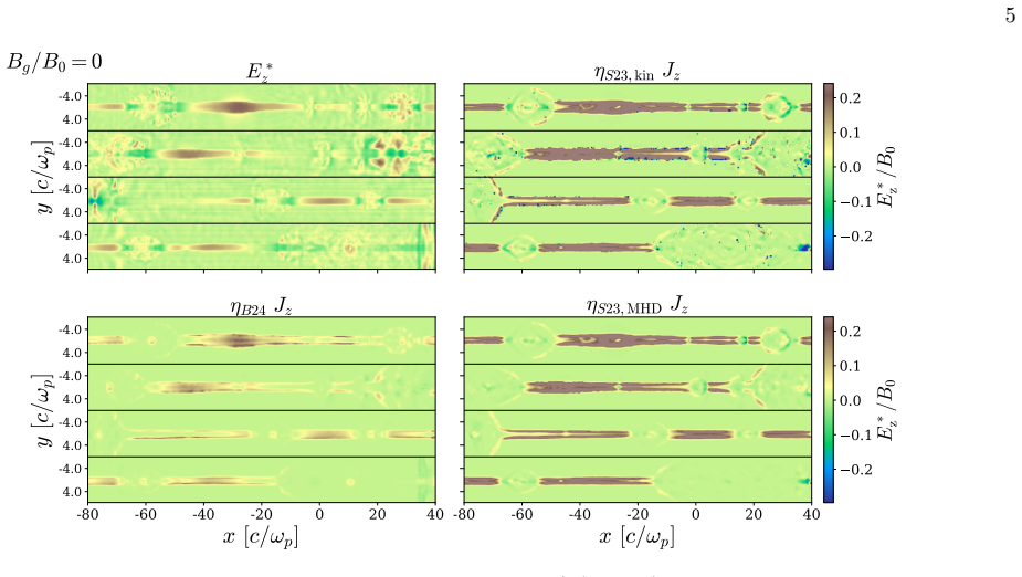
The paper's central discovery is an empirical prescription for the effective resistivity that captures the nonideal electric field in relativistic pair-plasma reconnection. For each guide field, the authors fit the two parameters $\alpha$ and $p$ by minimizing a weighted squared error between $\eta_{\mathrm{eff}} J_z$ and the directly measured $E^*_z$, and show that the same scalar resistivity also captures $E^*_x$ when a guide field is present. The fitted $p$ rises from near zero at zero guide field to roughly $18$ at $B_g/B_0 = 1$, and $\alpha/2$ tracks the measured reconnection rate. The reconstruction works not only in the main current layer but in the anti-reconnection layers between merging plasmoids, and it remains accurate in higher-resolution runs and in runs with strong synchrotron cooling. In the high-$p$ limit the formula reduces to $\eta_{\mathrm{eff}} \simeq |\mathbf{E}^*|/(e n_t c)$, which the paper argues is the most promising form to implement in resistive MHD because it has no free parameters and no guide-field dependence.
Load-bearing premise
The model assumes that the electric field breaking magnetic flux freezing can be captured locally by a single number multiplying the electric current, where that number depends only on the current's strength, the plasma density, and constants fit for the guide field.
Editorial extensions
If this is right
- Resistive MHD codes can replace uniform resistivity with this local, coordinate-agnostic formula, potentially raising reconnection rates from the uniform-resistivity value toward the kinetic value.
- Because the formula uses only the current density and the plasma number density, no spatial derivatives or species information are required, so it can be dropped into existing relativistic MHD codes regardless of grid orientation.
- For guide fields $B_g/B_0 \ge 0.3$, the high-$p$ limit $\eta_{\mathrm{eff}} \simeq |\mathbf{E}^*|/(e n_t c)$ removes both fitted parameters, making the prescription guide-field independent.
- The same scalar resistivity reproduces both the $z$ and $x$ components of the nonideal field, not just the component used for fitting.
- The fitted parameters carry over to higher-resolution runs and to runs with strong synchrotron cooling, indicating the prescription is not an artifact of the reference resolution or of radiative losses.
Reading between the lines
- The parameter-free high-$p$ limit suggests a deeper interpretation the paper only gestures at: the reconnection electric field is self-regulated by charge starvation, so any fluid model may effectively need to cap the current at roughly $e n_t c$. A useful test would be to see whether resistive-MHD runs with this prescription automatically keep $|\mathbf{J}| \lesssim e n_t c$.
- The success of an isotropic scalar resistivity implies that the pressure-tensor and inertial terms that actually mediate collisionless reconnection can be integrated out for global dissipation purposes. If that holds, simpler single-fluid simulations may capture flare energetics without two-fluid closures, at least for pair plasmas.
- The guide-field dependence of $p$ suggests that $p$ measures how much of the layer is charge-starved; extending the fits to lower magnetization and to electron-ion composition would reveal whether the $e n_t c$ normalization should be replaced by a species-weighted density.
Editorial analysis
A structured set of objections, weighed in public.
Referee Report
Summary. The paper proposes an empirical effective resistivity for relativistic pair-plasma reconnection, based on 2D PIC simulations with guide fields Bg/B0 = 0, 0.3, 0.6, and 1.0 at magnetization sigma = 50. The proposed form, Eq. (9)/(10), is local, coordinate-agnostic, and written in single-fluid MHD variables, with two fitted parameters alpha and p whose guide-field dependence is characterized. The authors show that the reconstruction eta_eff J reproduces the spatial structure of E*_z and E*_x in their PIC runs, and they recommend the high-p limit eta_eff = |E*|/(e n_t c), Eq. (14), as the most promising form for implementation in resistive MHD. The paper also reports robustness checks with higher resolution and synchrotron cooling, and it states caveats about 2D geometry, pair-plasma composition, and magnetization.
Significance. If the prescription held as an MHD closure, it would be a practically useful subgrid model: unlike the kinetically motivated forms of Selvi et al. (2023) and Bugli et al. (2024), it has no spatial derivatives, is independent of coordinate orientation, and is proposed for arbitrary guide-field strength. The paper is honest about its limitations and includes resolution and cooling checks. However, the recommended implementation in Eq. (14) is internally inconsistent as an Ohm's-law closure, and the fitted parameter p is only weakly constrained, so the guide-field dependence and the central promise of enhancing resistive-MHD reconnection rates are not yet established by the material presented.
major comments (3)
- [Section 5, Eq. (14)] Equation (14), recommended as 'the most promising form of effective resistivity to implement in resistive MHD simulations', is not a usable Ohm's-law closure. In a resistive MHD code the nonideal field is defined by E* = eta_eff J (Eq. 2). Inserting eta_eff = |E*|/(e n_t c) and taking the norm gives |E*| = |E*| |J|/(e n_t c). For any |J| != e n_t c the only solution is E* = 0, and at |J| = e n_t c any vector parallel to J satisfies the equation, so E* is undetermined. The finite-p model of Eq. (9) has a unique nonzero solution for |J| > 0, so the p -> infinity limit does not commute with the Ohm's-law solve. Equation (13) makes the difficulty explicit: eta_eff is expressed in terms of |E*|, an unknown that must be solved for. The recommended implementation therefore cannot be evaluated from single-fluid MHD variables, and no resistive-MHD run is provided to show that Eq. (14) enhances the reconnection rate. The authors should either recommend the explicit finite-p form (Eq. 9) and demonstrate it in a resistive MHD simulation, or present an implicit treatment of Eq. (14) that is shown to be well-posed.
- [Section 4, Tables 1 and 4; Appendix C] The loss function does not strongly constrain p. For Bg/B0 = 0 the best fit is p = 0 with an acceptable range [0.00, 1.73], yet Appendix C reports that p = 4, 8, and 10 give excellent reconstructions, and Section 5 recommends p >> 1; for Bg/B0 = 0.3 the acceptable interval is [4.22, 18.2]. Table 4 shows that changing p from pbest to phigh changes the L2 loss by less than about 10% for every guide field. Consequently the trend of pbest versus guide field in Fig. 6 is not robustly determined, and the claim that the guide-field dependence is encoded in alpha and p is not supported by the fits. This also undermines the physical interpretation that p distinguishes the zero-guide-field regime from higher guide fields.
- [Section 4 (fitting) and Section 5 (application)] All quantitative validation is in-sample. The parameters alpha and p are fit on the composite domain of the same PIC runs that are used for the spatial reconstructions in Figs. 7 and 8 and for the loss values in Table 4. The independent checks in Appendix A concern only zero guide field and are evaluated visually, without the loss metric. Since the abstract promises a strategy for enhancing the reconnection rate in resistive MHD simulations, the absence of any resistive-MHD run using the proposed prescription leaves the central application untested. I request at least one demonstration in a resistive MHD code, or a clear statement that the paper proposes but does not test the strategy.
minor comments (3)
- [Section 4, Eq. (11)] The summation in the loss function is written without an explicit index set; please specify that it runs over all cells in the composite domain and over all snapshots, and state the total number of cells and snapshots used for each guide-field case.
- [Section 3.2, Eq. (10)] The equivalence between Eq. (9) and Eq. (10) is stated without derivation; a one-line derivation would help readers verify that eta_eff = (alpha B0/|J|) / [1 + (c/|v_dr|)^(p+1)].
- [Figure captions] Figure 1 defines x = 0 as the edge of the simulation domain, while Figs. 3 and 7 measure x with respect to the center of the displayed portion; please standardize the coordinate description across captions to avoid confusion.
Circularity Check
The recommended high-p closure (Eq. 14) is self-referential and degenerate, and the α/2–reconnection-rate agreement is built into the ansatz rather than independently predicted.
-
self definitional
[Section 5, Equations 13–14]
"Our prescription in Equation 9 can be equivalently written as ηeff = (|E∗|/entc) [ (αB0 − |E∗|)/|E∗| ]^{1/(p+1)}. (13) In the limit of very high p, the square bracket is elevated to a very small power, yielding a contribution of order unity... ηeff ≃ |E∗|/entc (14)... We therefore regard Equation 14 as the most promising form of effective resistivity to implement in resistive MHD simulations of relativistic reconnection."
Equation 13 is not an approximation: combined with the defining Ohm law E∗ = ηeff J, the bracket equals (entc/|J|)^{p+1}, whose 1/(p+1) power is exactly entc/|J|, so Equation 13 merely restates ηeff = |E∗|/|J|. Inserting the recommended Equation 14 back into E∗ = ηeff J gives |E∗| = |E∗| |J|/(entc). For |J| ≠ entc the only solution is E∗ = 0; at |J| = entc the magnitude of E∗ is arbitrary. The finite-p model instead has a unique solution (E∗ → αB0 J/|J| for |J| > entc and E∗ → 0 below). The recommended parameter-free closure therefore does not predict the nonideal field; it reimposes the charge-starvation condition |J| = entc and leaves E∗ undetermined. This is a self-referential closure, not a derived limit of the model.
-
fitted input called prediction
[Section 3.2, Equations 8–9 and Figure 4]
"we expect that in regions of strong current... the nonideal electric field should approach |E∗| → (vin/c)B0 ... which implies that the effective resistivity should be ηeff → (vin/c) B0/|J|. (8)... We will determine free parameters α and p from PIC simulations. This scales as ηeff ∝ |J|p/(entc)p+1 at small currents and approaches ηeff = αB0/(2|J|) for |J| ≃ entc. We therefore expect α/2 ≃ vin/c, as we indeed find below (see also Figure 4)."
The ansatz in Equation 9 was deliberately constructed so that at |J| ≈ entc the resistivity becomes αB0/(2|J|). Since E∗z at the X-point equals (vin/c)B0 by the definition of the reconnection rate, fitting α to E∗z almost forces α/2 ≈ vin/c. The agreement shown in Figure 4 is therefore a built-in consistency check of the ansatz, not an independent confirmation that the prescription predicts the kinetic reconnection rate. The same E∗z data are used both to fit α,p and to infer vin, so the match is statistically and structurally forced.
full rationale
The paper's core empirical construction is an honest fit: α and p are fitted to E∗z with a weighted L2 loss (Equation 11), and the reconstruction ηeffJz is compared back to the same measured field. That in-sample reproduction is not by itself a circular prediction, and the paper does provide some out-of-sample checks (higher resolution, synchrotron cooling, the x-component of E∗, Appendices A and Figure 8). The comparison with Selvi et al. (2023) is a baseline model, not a load-bearing self-citation or uniqueness argument. The genuine circularity is in the recommended implementation. Equation 13 is an algebraic identity that reduces to ηeff = |E∗|/|J|; the claim that the bracket is of order unity holds only around |J| ≈ entc. Substituting the recommended Equation 14 into the defining Ohm law E∗ = ηeff J yields a degenerate equation whose only nonzero solutions sit at |J| = entc, with E∗ otherwise undetermined, so the parameter-free closure cannot be evaluated from single-fluid MHD variables as claimed. Relatedly, the α/2 ≈ vin/c agreement in Figure 4 is engineered by the ansatz in Equation 8 and the fit to E∗z, so it is a self-consistency check rather than evidence that the resistivity prescription independently predicts the reconnection rate. No resistive-MHD run is provided to demonstrate the claimed enhancement, and the stated caveats (2D geometry, pair composition, σ = 50) are honest but do not repair the self-referential character of Equation 14.
Assumptions & free parameters
free parameters (2)
- alpha =
0.3268, 0.1736, 0.1264, 0.0884 for Bg/B0 = 0.0, 0.3, 0.6, 1.0 (from alpha = m p + b in Table 2 at p = pbest)
- p =
0.00, 9.59, 15.4, 18.2 for Bg/B0 = 0.0, 0.3, 0.6, 1.0
assumptions (6)
- domain assumption The nonideal electric field in collisionless reconnection can be written as a scalar resistivity times the current, eta_eff J, within single-fluid relativistic MHD (Eq. 2).
- ad hoc to paper The functional form eta = alpha B0 |J|^p / (|J|^(p+1) + (e n_t c)^(p+1)) is an adequate ansatz for the effective resistivity.
- domain assumption The z-component of the nonideal field is sufficient to calibrate eta, and the same scalar eta applies to the other components.
- domain assumption Two-dimensional PIC simulations of pair-plasma reconnection capture the nonideal-field physics relevant for three-dimensional systems.
- ad hoc to paper The loss function L = sum |E*_z - eta J_z|^2 |E*_z| and the patch-selection rule (Eq. 12) lead to reliable parameter estimates.
- domain assumption The fitted alpha and p transfer without adjustment to runs with higher resolution and with synchrotron cooling.
Cite this review
Pith. "Pith review of Effective resistivity in relativistic reconnection: a prescription based on fully kinetic simulations." pith.science (2026). https://pith.science/paper/YZHUTYSO
@misc{pith2026250104800,
  author       = {Pith},
  title        = {Pith review of: Effective resistivity in relativistic reconnection: a prescription based on fully kinetic simulations},
  year         = {2026},
  howpublished = {\url{https://pith.science/paper/YZHUTYSO}},
  note         = {Machine review of arXiv:2501.04800}
}
abstract
A variety of high-energy astrophysical phenomena are powered by the release -- via magnetic reconnection -- of the energy stored in oppositely directed fields. Single-fluid resistive magnetohydrodynamic (MHD) simulations with uniform resistivity yield dissipation rates that are much lower (by nearly one order of magnitude) than equivalent kinetic calculations. Reconnection-driven phenomena could be accordingly modeled in resistive MHD employing a non-uniform, ``effective'' resistivity informed by kinetic calculations. In this work, we analyze a suite of fully kinetic particle-in-cell (PIC) simulations of relativistic pair-plasma reconnection -- where the magnetic energy is greater than the rest mass energy -- for different strengths of the guide field orthogonal to the alternating component. We extract an empirical prescription for the effective resistivity, $\eta_{\mathrm{eff}} = \alpha B_0 \mathbf{|J|}^p / \left(|\mathbf{J}|^{p+1}+\left(e n_t c\right)^{p+1}\right)$, where $B_0$ is the reconnecting magnetic field strength, $\bf J$ is the current density, $n_t$ the lab-frame total number density, $e$ the elementary charge, and $c$ the speed of light. The guide field dependence is encoded in $\alpha$ and $p$, which we fit to PIC data. This resistivity formulation -- which relies only on single-fluid MHD quantities -- successfully reproduces the spatial structure and strength of nonideal electric fields, and thus provides a promising strategy for enhancing the reconnection rate in resistive MHD simulations.
Figures


Figures from the paper (9 more)


Reference graph
Works this paper leans on
-
[1]
1943, Arkiv for Matematik, Astronomi och Fysik, 29B, 1
Alfv´ en, H. 1943, Arkiv for Matematik, Astronomi och Fysik, 29B, 1
work page 1943
-
[2]
2005, PhRvL, 95, 245001, doi: 10.1103/PhysRevLett.95.245001 —
Bessho, N., & Bhattacharjee, A. 2005, PhRvL, 95, 245001, doi: 10.1103/PhysRevLett.95.245001 —. 2007, Physics of Plasmas, 14, 056503, doi: 10.1063/1.2714020 —. 2010, Physics of Plasmas, 17, 102104, doi: 10.1063/1.3488963 —. 2012, ApJ, 750, 129, doi: 10.1088/0004-637X/750/2/129
-
[3]
Birn, J., Drake, J. F., Shay, M. A., et al. 2001, J. Geophys. Res., 106, 3715, doi: 10.1029/1999JA900449
-
[4]
2001, Physics of Plasmas, 8, 3282, doi: 10.1063/1.1377611
Biskamp, D., & Schwarz, E. 2001, Physics of Plasmas, 8, 3282, doi: 10.1063/1.1377611
-
[5]
2021, PhRvL, 127, 055101, doi: 10.1103/PhysRevLett.127.055101
Bransgrove, A., Ripperda, B., & Philippov, A. 2021, PhRvL, 127, 055101, doi: 10.1103/PhysRevLett.127.055101
-
[6]
Relativistic reconnection with effective resistivity: I. Dynamics and reconnection rate
Bugli, M., Lopresti, E. F., Figueiredo, E., et al. 2024, arXiv e-prints, arXiv:2410.20924, doi: 10.48550/arXiv.2410.20924
work page Pith review arXiv doi:10.48550/arxiv.2410.20924 2024
-
[7]
Cai, H. J., & Lee, L. C. 1997, Physics of Plasmas, 4, 509, doi: 10.1063/1.872178
-
[8]
Cassak, P. A., Liu, Y. H., & Shay, M. A. 2017, Journal of Plasma Physics, 83, 715830501, doi: 10.1017/S0022377817000666
Show all 40 references
-
[9]
2023, ApJ, 959, 122, doi: 10.3847/1538-4357/acffc6
Chernoglazov, A., Hakobyan, H., & Philippov, A. 2023, ApJ, 959, 122, doi: 10.3847/1538-4357/acffc6
2023 doi
-
[10]
2016, Journal of Plasma Physics, 82, 595820601, doi: 10.1017/S002237781600101X Del Zanna, L., Zanotti, O., Bucciantini, N., & Londrillo, P
Comisso, L., & Bhattacharjee, A. 2016, Journal of Plasma Physics, 82, 595820601, doi: 10.1017/S002237781600101X Del Zanna, L., Zanotti, O., Bucciantini, N., & Londrillo, P. 2007, A&A, 473, 11, doi: 10.1051/0004-6361:20077093
2016 doi
-
[11]
2019, PhRvL, 123, 225101, doi: 10.1103/PhysRevLett.123.225101
Egedal, J., Ng, J., Le, A., et al. 2019, PhRvL, 123, 225101, doi: 10.1103/PhysRevLett.123.225101
2019 doi
-
[12]
2023, PhRvL, 130, 115201, doi: 10.1103/PhysRevLett.130.115201
Galishnikova, A., Philippov, A., Quataert, E., et al. 2023, PhRvL, 130, 115201, doi: 10.1103/PhysRevLett.130.115201
2023 doi
-
[13]
2022, PhRvL, 129, 265101, doi: 10.1103/PhysRevLett.129.265101
Goodbred, M., & Liu, Y.-H. 2022, PhRvL, 129, 265101, doi: 10.1103/PhysRevLett.129.265101
2022 doi
-
[14]
2020, Physics of Plasmas, 27, 080501, doi: 10.1063/5.0012094
Guo, F., Liu, Y.-H., Li, X., et al. 2020, Physics of Plasmas, 27, 080501, doi: 10.1063/5.0012094
2020 doi
-
[15]
2024, SSRv, 220, 43, doi: 10.1007/s11214-024-01073-2
Guo, F., Liu, Y.-H., Zenitani, S., & Hoshino, M. 2024, SSRv, 220, 43, doi: 10.1007/s11214-024-01073-2
2024 doi
-
[16]
Harris, E. G. 1962, Il Nuovo Cimento, 23, 115, doi: 10.1007/BF02733547 12
1962 doi
-
[17]
2007, Physics of Plasmas, 14, 112102, doi: 10.1063/1.2801482
Hesse, M., & Zenitani, S. 2007, Physics of Plasmas, 14, 112102, doi: 10.1063/1.2801482
2007 doi
-
[18]
2016, Physics of Plasmas, 23, 080701, doi: 10.1063/1.4960669
Hirvijoki, E., Lingam, M., Pfefferl´ e, D., et al. 2016, Physics of Plasmas, 23, 080701, doi: 10.1063/1.4960669
2016 doi
-
[19]
1994, Physics of Plasmas, 1, 3587, doi: 10.1063/1.870894
Horiuchi, R., & Sato, T. 1994, Physics of Plasmas, 1, 3587, doi: 10.1063/1.870894
1994 doi
-
[20]
2012, SSRv, 173, 521, doi: 10.1007/s11214-012-9931-z
Hoshino, M., & Lyubarsky, Y. 2012, SSRv, 173, 521, doi: 10.1007/s11214-012-9931-z
2012 doi
-
[21]
2015, Space Science Reviews, 191, 545, doi: 10.1007/s11214-014-0132-9
Kagan, D., Sironi, L., Cerutti, B., & Giannios, D. 2015, Space Science Reviews, 191, 545, doi: 10.1007/s11214-014-0132-9
2015 doi
-
[22]
Komissarov, S. S. 2007, MNRAS, 382, 995, doi: 10.1111/j.1365-2966.2007.12448.x
2007
-
[23]
Kulsrud, R. M. 1998, Physics of Plasmas, 5, 1599, doi: 10.1063/1.872827 —. 2001, Earth, Planets and Space, 53, 417, doi: 10.1186/BF03353251
1998 doi
-
[24]
M., Hesse, M., & Winske, D
Kuznetsova, M. M., Hesse, M., & Winske, D. 1998, J. Geophys. Res., 103, 199, doi: 10.1029/97JA02699
1998 doi
-
[25]
2017, Physics of Plasmas, 24, 042120, doi: 10.1063/1.4980838
Bhattacharjee, A. 2017, Physics of Plasmas, 24, 042120, doi: 10.1063/1.4980838
2017 doi
- [26]
-
[27]
R., & Pridmore-Brown, D
Lyons, L. R., & Pridmore-Brown, D. C. 1990, J. Geophys. Res., 95, 20903, doi: 10.1029/JA095iA12p20903
1990 doi
-
[28]
Favre, J. M. 2014, A&A, 570, A111, doi: 10.1051/0004-6361/201424083
2014 doi
-
[29]
2019, MNRAS, 485, 299, doi: 10.1093/mnras/stz387
Ripperda, B., Porth, O., Sironi, L., & Keppens, R. 2019, MNRAS, 485, 299, doi: 10.1093/mnras/stz387
2019 doi
-
[30]
2023, ApJ, 950, 169, doi: 10.3847/1538-4357/acd0b0
Selvi, S., Porth, O., Ripperda, B., et al. 2023, ApJ, 950, 169, doi: 10.3847/1538-4357/acd0b0
2023 doi
-
[31]
2022, PhRvL, 128, 145102, doi: 10.1103/PhysRevLett.128.145102
Sironi, L. 2022, PhRvL, 128, 145102, doi: 10.1103/PhysRevLett.128.145102
2022 doi
-
[32]
2014, ApJL, 783, L21, doi: 10.1088/2041-8205/783/1/L21
Sironi, L., & Spitkovsky, A. 2014, ApJL, 783, L21, doi: 10.1088/2041-8205/783/1/L21
2014 doi
-
[33]
2005, in American Institute of Physics Conference Series, Vol
Spitkovsky, A. 2005, in American Institute of Physics Conference Series, Vol. 801, Astrophysical Sources of High Energy Particles and Radiation, ed. T. Bulik, B. Rudak, & G. Madejski (AIP), 345–350, doi: 10.1063/1.2141897
2005 doi
-
[34]
R., Zenitani, S., Matsukiyo, S., et al
Totorica, S. R., Zenitani, S., Matsukiyo, S., et al. 2023, ApJL, 952, L1, doi: 10.3847/2041-8213/acdb60
2023 doi
-
[35]
2003, in APS Meeting Abstracts, Vol
Uzdensky, D. 2003, in APS Meeting Abstracts, Vol. 45, APS Division of Plasma Physics Meeting Abstracts, BO2.003
2003
-
[36]
A., Loureiro, N
Uzdensky, D. A., Loureiro, N. F., & Schekochihin, A. A. 2010, PhRvL, 105, 235002, doi: 10.1103/PhysRevLett.105.235002
2010 doi
-
[37]
R., & Uzdensky, D
Werner, G. R., & Uzdensky, D. A. 2017, ApJL, 843, L27, doi: 10.3847/2041-8213/aa7892
2017 doi
-
[38]
2010, ApJL, 716, L214, doi: 10.1088/2041-8205/716/2/L214
Zenitani, S., Hesse, M., & Klimas, A. 2010, ApJL, 716, L214, doi: 10.1088/2041-8205/716/2/L214
2010 doi
-
[39]
2021, ApJ, 922, 261, doi: 10.3847/1538-4357/ac2e08
Zhang, H., Sironi, L., & Giannios, D. 2021, ApJ, 922, 261, doi: 10.3847/1538-4357/ac2e08
2021 doi
-
[40]
Zhang, H., Sironi, L., Giannios, D., & Petropoulou, M. 2023, ApJL, 956, L36, doi: 10.3847/2041-8213/acfe7c 13 -2.0 2.0 -2.0 2.0 -2.0 2.0 -2.0 2.0 y [c/ωp] E ∗ z ηS23, kin Jz ηS23, MHD Jz 0.4 0.2 0.0 0.2 -40 -30 -20 -10 0 10 20 30 40 x [c/ωp] -2.0 2.0 -2.0 2.0 -2.0 2.0 -2.0 2.0...
2023 doi
Reviewed August 10, 2026 · model on record in the stance chip above.
Discussion (0). Continue with ORCID to comment.