REVIEW 4 major objections 5 minor 1 cited by
Marketron games: Self-propelling stocks vs dumb money and metastable dynamics of the Good, Bad and Ugly markets
T0 review · 4 major / 5 minor · reviewed 2026-08-10 · deepseek-v4-flash
Pith's one-line read A money-flow feedback loop can generate three metastable market regimes, including crashes and defaults, without jumps or separate default processes.
desk verdict A genuinely new 2D marketron model with memory and real calibration effort, but the three-regime claim is enforced by constraints whose derivation fails at the fitted parameters. read the letter →
The pith
A machine-rendered reading of the paper's core claim, the machinery that carries it, and where it could break.
The reading
What carries the argument
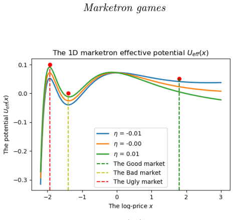
The machinery is the marketron potential $V(x,y)=-\eta x + c(t)y\,V_M(x)+\frac{1}{2\mu}(y-\bar y)^2$, whose $x$-gradient drives the log-price and whose $y$-gradient drives the memory variable. The flow potential $V_M(x)$ is approximated by an inverted Morse potential, and in the D-limit of zero noise, zero signal, and short memory the memory variable is slaved to $x$, leaving the effective one-dimensional potential $U_{\rm eff}(x)=-\eta x + c(t)\bar y\,V_M(x)-\frac{c(t)^2}{2\mu}V_M^2(x)$. Appendix C imposes constraints on the quartic $zV'(z)$ to guarantee four real roots and hence three extrema, which are the Good, Bad, and Ugly states. Instantons, defined as trajectories of the inverted potential that dominate the weak-noise path integral, convert barrier crossings into fast transitions between these metastable states, which is what makes crashes and defaults rare but possible.
What would settle it
Recalibrate Eq. (29) to S&P500 daily returns without imposing the Appendix C constraints; if a moment-matching solution exists whose potential has fewer than three extrema, or whose simulated default intensity falls far outside the 10-50 basis point range, then the three-regime metastable structure and the 18 basis point default reading are consequences of the constraints rather than of the money-flow mechanism.
Extended reading notes
Core claim
The central claim is that price dynamics in an inelastic market can be represented as nonlinear diffusion of a marketron in a two-dimensional potential $V(x,y)=-\eta x + c(t)y\,V_M(x)+\frac{1}{2\mu}(y-\bar y)^2$, where $x$ is the log-price and $y$ is a memory variable storing past money flows. When money flows respond positively to market performance, the coupling between $y$ and the inverted-Morse flow potential creates barriers, so the potential has three extrema. The right minimum is the Good market, the middle minimum is the Bad market, and the maximum with an escape route to $x\to-\infty$ is the Ugly market. Transitions between these states are instanton solutions of the flipped-potential dynamics, making the regimes metastable. Calibrating the three-dimensional version to S&P500 monthly log-prices under shape constraints reproduces the skewness and kurtosis of log-returns and produces defaults at a rate of about 18 basis points, which the paper presents as evidence that defaultability emerges from money-flow feedback rather than from an added jump process.
Load-bearing premise
The load-bearing premise is that the small-noise memory-variable approximation behind the constraints in Eq. (30) is accurate enough that forcing the quartic $zV'(z)$ to have four real roots genuinely yields the Good/Bad/Ugly landscape rather than an artifact; if the $y$-noise is strong, those constraints become stochastic and the calibrated three-regime structure is no longer guaranteed.
Editorial extensions
If this is right
- Equity defaults and market crashes require no jump process or exogenous default intensity; they arise as instanton escapes through barriers created by the money-flow feedback loop.
- The calibrated model reproduces the negative skew and positive excess kurtosis of S&P500 log-returns across horizons from 2 to 24 years.
- Simulated paths of the calibrated model generate an annualized default intensity near 18 basis points, within the 10-50 basis point range inferred from credit markets, using only equity data.
- Because the model is Markovian in $(x,y,\theta)$ but non-Markovian in price alone, volatility clustering and price-volatility correlations emerge from the memory variable rather than from an external stochastic-volatility process.
Reading between the lines
- Pith inference: The model turns equity and credit into two readings of one parameter set; joint calibration to equity returns and CDS spreads could tighten the 10-50 basis point default intensity band and test the physical-to-credit link.
- Pith inference: Treating the unobservable OU signals as self-propulsion suggests that optimal investor policies could be derived as minimum-cost controls of an active particle in the Good/Bad/Ugly landscape, not merely calibrated.
- Pith inference: A direct test would replace the shape constraints with unconstrained calibration to daily returns and check whether three extrema persist; if they disappear, the metastable structure is an artifact of the constraints rather than a prediction.
Signed reviews
Editorial analysis
A structured set of objections, weighed in public.
Referee Report
Summary. This paper proposes a two-dimensional Langevin ('marketron') model of price formation in which the log-price x and a memory variable y evolve under a potential V(x,y) = -ηx + c(t)y V_M(x) + (1/(2μ))(y - ȳ)^2 (Eqs. 18 and 20). The memory variable encodes past money flows, and an unobserved OU signal z is reinterpreted as an active self-propulsion force. In the D-limit μ >> 1 the model reduces to a 1D effective potential (Eq. 26) and is claimed to produce three metastable market regimes—Good, Bad, Ugly—with instanton transitions. The model is calibrated to S&P 500 monthly log-returns using a particle filter with shape constraints (Eq. 30); the calibrated model matches the first four moments of log-returns across horizons and produces an annualized default intensity of about 18 bps without exogenous jumps.
Significance. If the three-regime landscape were emergent, the paper would be a substantial contribution: it offers a parsimonious nonlinear mechanism for crashes and defaults, connects flow impact to metastability, and provides a transparent calibration with explicit parameters, seeds, and constraints. The strengths include the internally consistent 2D potential algebra, the explicit reporting of all 18 calibrated parameters in Tables 1 and 4, and the reproducible calibration protocol. However, the empirical identification of the three regimes is undermined by the fact that the constraints in Eq. (30) are imposed during calibration, and the approximations used to derive them are violated by the calibrated parameters. The 18 bps default intensity can therefore not yet be read as an independent confirmation of the metastable landscape.
major comments (4)
- [§6, Appendix C, Eq. (30)] The three-regime structure is enforced, not predicted. The text states that the constraints 'explicitly require the calibrated parameters to preserve the necessary shape', and Eq. (30) are derived in Appendix C as necessary conditions for the quartic zV'(z) to have four real roots. Figures 16 and 17 therefore show only that the calibration constraints were satisfied. To support the claim that the model 'predicts' Good/Bad/Ugly regimes, please add an unconstrained calibration and report the shape of the resulting potential, or explicitly reframe the regime structure as part of the model specification and revise the abstract and Section 7 accordingly.
- [Appendix C, Eq. (C.12)] The stochastic correction to the constraints is invalid. The derivation drops σ_y from the y-SDE; with σ_y > 0, y(0) is replaced by y(0) - σ_y∫... in Eq. (C.11). The assertion in Eq. (C.12) that y(0) >> σ_y times the martingale is 'always true on average' does not hold: since the calibration sets y(0) = 0 (Section 6.2), the required inequality is M_t << 0, and a zero-mean martingale does not satisfy this almost surely. Moreover, Table 1 gives σ_y = 0.38, comparable to σ = 0.79, so the small-noise premise is violated. Consequently, the calibrated parameters do not provably yield a three-extremum potential in the full stochastic model.
- [§3.1, Eq. (25)] The D-limit approximation (Eq. 25) requires μ >> 1, but the qualitative figures (Figs. 2-6) use μ = 0.1, and the calibrated values are μ = 1.67 and μ = 1.40 (Tables 1 and 4). The 1D potential U_eff (Eq. 26) and the Good/Bad/Ugly taxonomy derived from it are therefore not justified for these parameters. Please quantify the error of the D-limit at the calibrated parameters, for example by comparing 1D and 2D stationary densities or escape rates.
- [§6.2.1, default intensity] The annualized default intensity of about 18 bps is obtained from Monte Carlo simulation of the full 3D model using parameters selected under the constraints of Eq. (30). Given the issues with Eq. (C.12) and the small-noise premise, this number does not by itself validate the metastable barrier picture. Please compute the default intensity with unconstrained parameters, or at least verify the four-root condition with the full stochastic y-process, and report the resulting intensity.
minor comments (5)
- [Section 6.2] The sentence 'we use x0 = x(0), θ0 = y(0) = 0, y0 = y(0)' is ambiguous about the initial values; please state y0 and θ0 separately and consistently with Eq. (C.12).
- [Eq. (C.12)] The integrand is written with ε_t inside an integral over k; the noise should depend on the integration variable (e.g., ε_k), and the integral should be defined precisely.
- [Footnote 7] The inequality '0≥S≤∞' should read '0≤S≤∞'.
- [Table 3] The table labels kurtosis as 'annualized', but excess kurtosis is scale-invariant in this context; please clarify the reported quantity.
- [References] The reference 'Alt-Sahalia, Y.' should be 'Aït-Sahalia, Y.'.
Circularity Check
Three 'predicted' market regimes are imposed by the Eq. (30) calibration constraints; the Appendix C stochastic correction used to justify them is asserted away with an invalid martingale bound.
-
self definitional
[Section 6, Eq. (30); Section 6.2.1 'The marketron potential shape' (Figs. 16-17)]
"Since this paper is focused on situations where the marketron potential has a form as in Fig. 6 (where transitions between various regimes occur via the instanton mechanism), additional constraints should be imposed when performing filtering because not every calibration gives rise to this form of potential. ... By adding an additional constraint as in Appendix C, we explicitly require the calibrated parameters to preserve the necessary shape. ... Accordingly, the potential has three extrema, i.e., exactly what we tried to achieve."
The three-regime landscape is not an emergent output of the model: the optimizer is explicitly constrained to the region of parameter space where zV'(z) has four real roots, which is exactly the condition for the potential to have three extrema. The paper's own words confirm this ('we explicitly require the calibrated parameters to preserve the necessary shape' and 'exactly what we tried to achieve'). Any feasible solution of the constrained calibration therefore displays Good/Bad/Ugly structure by construction. The abstract's claim that the model 'predicts three distinct regimes' is thus a restatement of the imposed constraints, not an independent prediction.
-
other
[Appendix C, Eqs. (C.11)-(C.12)]
"In this case the constraint in Eq. (C.9) becomes stochastic, and it is not obvious how it can be used in the filtering method. Therefore, we impose an additional constraint that reads y(0)≫σy∫t0 ekµϵtdk = σy(Wteµt−1µ∫t0 Wkekµdk). The RHS of this inequality is a martingale, therefore, on average, it is always true."
This assertion is used to justify neglecting the y-noise when deriving the four-root constraints of Eq. (30). But the RHS is a zero-mean martingale, so its expectation is zero at every t; with the calibration's y(0)=0, the inequality 0 ≫ 0 is false on average, not 'always true'. The phrase 'on average' cannot control the pathwise magnitude of the noise that enters the actual filter. Since Eq. (30) is the only mechanism that enforces the three-extrema landscape, and the calibrated σy=0.38 is comparable to σ=0.79 (Table 1), the central regime claim rests on a stochastic correction that is asserted away rather than derived.
full rationale
The Langevin construction in Eqs. (12)-(23) is internally coherent as a model specification, and the calibration to S&P500 moment data is a legitimate fitting exercise. The circularity is concentrated in the paper's central claim. Section 6 explicitly constrains calibration to parameters that preserve a three-extrema potential shape, and Section 6.2.1 then reports the presence of three extrema as the result the authors 'tried to achieve.' The 18 bps default intensity and metastable regime dynamics are simulated with this enforced landscape, so they do not independently validate the Good/Bad/Ugly prediction. Appendix C's attempt to extend the four-root constraints beyond small y-noise fails because the inequality y(0)≫(zero-mean martingale) is not 'always true on average'—especially with y(0)=0 and σy=0.38. No load-bearing self-citation chain was found; prior Halperin/Dixon work is used as modeling background, not as a uniqueness theorem. Overall, the central 'prediction' is better described as a constrained calibration result, meriting a circularity score of 8.
Assumptions & free parameters
free parameters (10)
- g (coupling constant) =
0.6831 (Table 1)
- c (money flow scale) =
3.9305 (Table 1)
- mu (memory depth) =
1.6671 (Table 1)
- ybar (threshold) =
0.4731 (Table 1)
- eta (risk-adjusted drift) =
-1.5685 (Table 1)
- sigma, sigma_y, sigma_z (noise levels) =
0.7912, 0.3800, 0.8334 (Table 1)
- k (mean reversion of signal) =
1.2869 (Table 1)
- thetabar (signal mean level) =
6.7865 (Table 1)
- b1, b2, k1x, k2x, k3x, k1y, k2y, k3y (signal shape parameters) =
Various, Table 1
- epsilon (regularization parameter) =
0.02 (fixed, Section 6.2)
assumptions (7)
- standard math Itô's lemma and standard stochastic calculus are used to transform the price SDE into log-price dynamics.
- domain assumption The investor policy ut = c(t) S0 [1 - g/(e^x + epsilon g)] is a posited functional form, not derived from utility optimization.
- ad hoc to paper The price impact function I = y_t u_t/S_t with memory variable y_t is assumed, and the potential V(y) is chosen so that the y-dynamics reproduce an EMA of flows.
- domain assumption Return predictors are unobservable OU processes (Eq. 6), interpreted as self-propulsion; this interpretation does not change the mathematics but is presented as the active matter analogy.
- ad hoc to paper The calibration imposes the shape constraints in Eq. (30) which guarantee four roots of the quartic, hence three extrema of the potential.
- ad hoc to paper The D-limit approximation y_t = ybar + (c/mu) V_M(x) assumes mu >> 1, but is used with mu = 0.1 in qualitative plots.
- domain assumption The approximate inverted-Morse potential Eq. (19) is used for qualitative analysis and in the constraint derivation.
invented entities (2)
-
Memory variable y_t
-
Marketron quasi-particle
Cite this review
Pith. "Pith review of Marketron games: Self-propelling stocks vs dumb money and metastable dynamics of the Good, Bad and Ugly markets." pith.science (2026). https://pith.science/paper/QJGZ37DY
@misc{pith2026250112676,
  author       = {Pith},
  title        = {Pith review of: Marketron games: Self-propelling stocks vs dumb money and metastable dynamics of the Good, Bad and Ugly markets},
  year         = {2026},
  howpublished = {\url{https://pith.science/paper/QJGZ37DY}},
  note         = {Machine review of arXiv:2501.12676}
}
abstract
We present a model of price formation in an inelastic market whose dynamics are partially driven by both money flows and their impact on asset prices. The money flow to the market is viewed as an investment policy of outside investors. For the price impact effect, we use an impact function that incorporates the phenomena of market inelasticity and saturation from new money (the $dumb \; money$ effect). Due to the dependence of market investors' flows on market performance, the model implies a feedback mechanism that gives rise to nonlinear dynamics. Consequently, the market price dynamics are seen as a nonlinear diffusion of a particle (the $marketron$) in a two-dimensional space formed by the log-price $x$ and a memory variable $y$. The latter stores information about past money flows, so that the dynamics are non-Markovian in the log price $x$ alone, but Markovian in the pair $(x,y)$, bearing a strong resemblance to spiking neuron models in neuroscience. In addition to market flows, the model dynamics are partially driven by return predictors, modeled as unobservable Ornstein-Uhlenbeck processes. By using a new interpretation of predictive signals as $self$-$propulsion$ components of the price dynamics, we treat the marketron as an active particle, amenable to methods developed in the physics of active matter. We show that, depending on the choice of parameters, our model can produce a rich variety of interesting dynamic scenarios. In particular, it predicts three distinct regimes of the market, which we call the $Good$, the $Bad$, and the $Ugly$ markets. The latter regime describes a scenario of a total market collapse or, alternatively, a corporate default event, depending on whether our model is applied to the whole market or an individual stock.
Figures


Figures from the paper (18 more)



Forward citations
Cited by 1 Pith paper
-
Non-Linear and Meta-Stable Dynamics in Financial Markets: Evidence from High Frequency Crypto Currency Market Makers
High-frequency Uniswap v3 crypto data show non-quadratic potentials, with double-well shapes at short sampling frequencies that the author links to market stress.
Reference graph
Works this paper leans on
-
[1]
If ∆> 0 and P <0,D< 0, then all four roots are real and distinct
-
[2]
If ∆ = 0 and P <0,D< 0, ∆0̸= 0, then there are a real double root and two real simple roots
-
[3]
If ∆< 0 there are two distinct real roots and two complex conjugate roots. Computing the RHS of Eq. (C.7) with allowance for the definitions in Eq. (C.6) yields ∆ = 1 16c(t)3g2J(t) { c(t)3g2I(t)4[J(t)− 2gI(t)] + 16c(t)¯η2g2J(t) [ −2g2I(t)2− 2gI(t)J(t) +J(t)2 ] − 4c(t)¯η [ c(t)g4I(t)4 + 2g2I(t)2J(t) [3c(t)gI(t) + 2] + 8J(t)3 [3c(t)gI(t) + 2] (C.9) + 2gI(t)...
Reviewed August 10, 2026 · model on record in the stance chip above.
Discussion (0). Continue with ORCID to comment.