REVIEW 5 major objections 6 minor 1 cited by
Mapping H$\alpha$-Excess Candidate Point Sources in the Southern Hemisphere Using S-PLUS Data
T0 review · 5 major / 6 minor · reviewed 2026-08-10 · deepseek-v4-flash
Pith's one-line read S-PLUS data yield 6,956 candidate H-alpha-excess point sources in the southern sky.
desk verdict A useful southern-sky candidate catalogue, with a load-bearing GDS locus assumption and circular ML validation that a revision should fix. read the letter →
The pith
A machine-rendered reading of the paper's core claim, the machinery that carries it, and where it could break.
The reading
What carries the argument
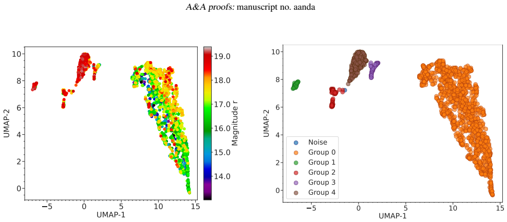
The central machinery is the (r−J0660) versus (r−i) colour-colour excess criterion: a linear fit to the stellar locus per field and magnitude bin, refined by iterative sigma clipping, defines the expected colour of a source without H-alpha; the selection condition (r−J0660)obs − (r−J0660)fit ≥ 5·σest flags candidates, where σest combines the fit scatter with the photometric errors of both colours. For the Galactic Disk Survey the iterative fit is moved upward toward the unreddened main sequence to handle differential reddening. Classification uses UMAP dimensionality reduction on 66 S-PLUS colour indices followed by HDBSCAN clustering, with a second pass adding two infrared bands to make 77 colours; a Random Forest trained on the cluster labels ranks the colours and provides the basis for simplified colour-colour cuts.
What would settle it
Randomly select a few hundred candidates from each survey and take optical spectra, counting the fraction with an emission or absorption feature inside J0660; if that fraction falls far below the paper's quoted roughly 60% emission plus 30% absorption among spectral matches, the 5-sigma locus criterion is not selecting what it claims. Re-running the fit with the threshold varied from 3 to 7 sigma should also change the candidate counts smoothly, not in a cliff that would signal an unstable fitted locus.
Extended reading notes
Core claim
The central claim is that H-alpha-excess point sources over the southern sky can be identified from S-PLUS DR4 photometry and grouped into astrophysical classes using colours alone. In the (r−J0660) versus (r−i) plane, non-emitting stars define a locus; the authors fit a line to that locus in each field and magnitude bin with iterative sigma clipping, then flag any source lying at least five estimated standard deviations above the fit. In crowded Galactic-disk fields with two loci produced by differential reddening, the fit is iterated upward to the presumed unreddened main sequence. Cross-matches show the selected objects are emission-line stars, young stellar objects, binaries, cataclysmic variables, planetary nebulae, RR Lyrae stars, quasars, and active galactic nuclei; for some quasars the J0660 excess is actually Mg II, C III], C IV, [O III], or H-beta redshifted into the filter. Clustering on 66 S-PLUS colours separates a quasar/AGN-dominated group from a group of RR Lyrae stars and binaries, and adding infrared colours resolves the cataclysmic-variable/quasar confusion. The authors deliberately call the sources 'H-alpha-excess' rather than 'H-alpha emitters,' since absorption lines and variability can produce the same photometric signature.
Load-bearing premise
The candidate list rests on the fitted lines in the (r−J0660) versus (r−i) plane tracing the colours of genuinely non-emitting stars, and, in the Galactic Disk Survey, on the upper locus being the unreddened main sequence; if reddening or calibration shifts those fits, the 5-sigma criterion adds contaminants or drops real emitters.
Editorial extensions
If this is right
- The 6,956-entry catalogue gives southern-sky surveys a compact point-source list for spectroscopic follow-up of H-alpha-excess candidates.
- Any S-PLUS field with clean photometry can be processed with the same per-field locus fit, so the method extends to future S-PLUS data releases.
- RR Lyrae stars and eclipsing binaries will keep appearing in sequential narrowband H-alpha selections because phase sampling and H-alpha absorption mimic excess; the paper shows how to recognise that population.
- Quasars and AGN at particular redshifts masquerade as H-alpha emitters when Mg II, C III], C IV, [O III], or H-beta lands in J0660, so infrared colours are needed to separate extragalactic from Galactic candidates.
- The simplified colour-colour diagrams distilled from the clustering allow pre-classification with a few filters, reducing the need for complete 12-band photometry.
Reading between the lines
- The same per-field locus-fitting procedure should transfer to the northern-sky twin survey with the same filter set; a direct test is cross-matching the colour criteria in overlap regions.
- Because the 5-sigma threshold is fixed and estimated per field, catalogue purity and completeness are likely patchy; a continuous probabilistic excess score would give each candidate an individual confidence.
- The clean separation of RR Lyrae stars suggests the 12-filter sequence itself encodes short-period variability information, which could be mined for variability beyond the H-alpha-excess sample.
- The remaining optical-only confusion between cataclysmic variables and quasars at z ~ 1.35 marks a boundary for photometric classification that infrared colours only partly resolve; adding other line-sensitive bands could push it further.
Signed reviews
Editorial analysis
A structured set of objections, weighed in public.
Referee Report
Summary. The paper presents a search for Hα-excess point sources in S-PLUS DR4 using the (r−J0660) versus (r−i) colour-colour method of Witham et al. (2008). The authors first apply iterative linear fits to the stellar locus in each field and magnitude bin for the Main Survey (MS) and the Galactic Disk Survey (GDS), selecting sources that lie at least 5σ above the fit. They report 6,956 candidates, 3,637 from the MS and 3,319 from the GDS, and cross-match them with SIMBAD, SDSS, LAMOST, and VPHAS+. They then use UMAP plus HDBSCAN to cluster the MS candidates, first with 66 S-PLUS colours and then with 77 colours including WISE W1/W2, and train a Random Forest on the cluster labels to identify important colours. The paper concludes that the S-PLUS 12-filter system can separate RR Lyrae stars and eclipsing binaries from genuine Hα emitters, that optical plus infrared data improve the separation of Galactic from extragalactic sources, and that the proposed colour-colour diagrams provide tentative pre-classification criteria.
Significance. If the candidate catalogue is sound, this work would provide a new southern-sky list of Hα-excess point sources and demonstrate the utility of S-PLUS narrow-band J0660 photometry for finding emission-line objects and variables. The paper has several genuine strengths: the selection procedure is described in enough detail to be followed; the SDSS and LAMOST spectra in Figs. 7–10 convincingly show that at least some selected objects are genuine emitters, CVs, and QSOs with redshifted lines; and the authors are explicit about contamination by RR Lyrae and eclipsing binaries and about caution for r<13.5 mag. However, the central catalogue is not actually included or linked, the GDS selection depends on an unverified choice of the 'upper locus' as the unreddened main sequence, and the Random Forest validation is circular with respect to physical classification because it is trained on HDBSCAN labels generated from the same photometric features. These issues currently prevent the reader from independently checking the headline numbers or the physical interpretation of the clusters.
major comments (5)
- [3.3 (Eq. 1, Fig. 5)] The GDS upper-locus fit is the load-bearing step for the 3,319 GDS candidates. The text states that the upper locus 'generally corresponds to the unreddened main sequence' but never demonstrates this by overlaying the Pickles main-sequence and giant tracks shown in Figs. 2–3 on a GDS field. Because the iterative procedure re-fits points above the initial line, genuine Hα emitters can drag the fitted line upward, and if the upper locus is in fact a reddened or giant-dominated population, Eq. (1) thresholds shift for every GDS source. The procedure is also not fully specified: the clipping threshold is described only as 'several σ' and the iteration count as '2 to 3'. Please overlay the Pickles tracks on representative GDS fields, quantify the offset between the initial and final fits per field and magnitude bin, specify the clipping algorithm precisely, and report how the 3,319-candidate count changes if the lower (reddened) locus is used as the reference.
- [4 and 6] The central catalogue is not provided. The headline result of the paper is a list of 6,956 Hα-excess candidates, but the manuscript contains no machine-readable table, no VizieR/CDS link, and no appendix table with candidate positions, photometry, errors, and flags. Without the catalogue, readers cannot verify the reported counts, the SIMBAD cross-match statistics, or the clustering metadata. Please add a full catalogue, ideally at CDS/VizieR, and describe its columns, duplicate handling, and provenance.
- [5.3 (Fig. 18, Fig. 19, Table 3)] The Random Forest validation is circular with respect to physical classification. The model is trained on HDBSCAN labels generated from the same 66–77 photometric colours used as input features, so the reported F1 macro average of 0.95 and the feature importances quantify how well the Random Forest reproduces the cluster labels, not whether the clusters correspond to physically distinct source classes. This circularity also affects the interpretation of Groups 0–4 in Table 3 and the tentative colour cuts in Fig. 19. Please either reframe Section 5.3 as an analysis of cluster-label reproducibility or validate the clusters against external spectroscopic classifications, reporting per-class precision and recall for confirmed CVs, QSOs, RR Lyrae stars, and eclipsing binaries.
- [4.3] The spectroscopic confirmation rates are not defined on a well-posed sample. The paper states that 'approximately 60%' of the 212 SDSS/LAMOST matches show emission lines and 'around 30%' show Hα absorption, but the denominator, the selection function, and any spectral signal-to-noise or line-strength thresholds are not given. The SDSS and LAMOST overlaps are not a random subsample of the candidate list, so these percentages cannot be interpreted as purity estimates for the full catalogue. Please provide a per-survey table of spectral classifications (emission, absorption, no line, unknown) and, if possible, report confirmation rates for a randomly selected or completeness-weighted subsample.
- [4.4 (Fig. 11)] The VPHAS+ comparison does not validate the candidate selection. The 793 matched objects are used to compare r−i and r−Hα colour differences between S-PLUS and VPHAS+, yielding medians of −0.21 and +0.02 with MADs of 0.07 and 0.27, but this does not test whether S-PLUS Hα-excess candidates coincide with VPHAS+ Hα-excess sources. A meaningful external check would cross-match the S-PLUS GDS candidate list with VPHAS+ photometry and compare the Hα-excess flags, reporting the fraction of S-PLUS candidates that are also VPHAS+ emitters and vice versa.
minor comments (6)
- [Header] The manuscript header contains placeholder dates ('Received September 15, 1996; accepted March 16, 1997') that should be corrected before submission.
- [Section 4 and Fig. 6] The filter is repeatedly written as 'J0600' in Section 4 and in the caption of Fig. 6; it should be 'J0660' consistently throughout the paper.
- [Fig. 19] The colour-colour diagrams in Fig. 19 are difficult to use because the pairplot panels lack clear axis labels and the tentative colour cuts are not legible in the printed figure; please replot with labelled axes and a legend for the cuts.
- [Section 5.2.1] The sentence 'We ended up with the optimal value of 2 and 50, respectively' does not specify which HDBSCAN parameter is 2 and which is 50; the order for min_samples and min_cluster_size should be stated explicitly.
- [Section 5.2.2] The text 'typically exhibit amplitudes higher than 0.3 to 2 magnitudes for RR Lyrae stars Chandra X-ray Observatory' contains what appears to be a citation placeholder; please replace it with proper references for RR Lyrae periods and amplitudes.
- [Section 2] There are several grammar and typographical slips, such as 'we primary goal of identify objects' in Section 2 and 'dmax,pro j' in Section 4; these should be corrected in a copy-editing pass.
Circularity Check
The Hα-excess catalogue is an independent empirical selection, but the machine-learning feature-importance and tentative colour-cut results are circular because the Random Forest is trained on HDBSCAN labels generated from the same photometric colours it is then used to 'discover'.
-
fitted input called prediction
[Section 5.3, 'Extracting Main Features: Colour Analysis', and Figure 19]
"We used the classifications made by combining UMAP and HDBSCAN to create Random Forest (Breiman 2001) models and identified the most important features, specifically the colours that contribute to the separation or classification of the classes of objects. ... using 66 S-PLUS colours plus 11 additional colours generated with the W1 and W2 filters as input parameters, and labels generated by HDBSCAN. ... Tentative colour cuts are presented in the Fig. 19 to differentiate the various classes of Hα sources."
The HDBSCAN cluster labels are produced by UMAP embeddings of the same 66 (or 77) photometric colours that are later used as input features to the Random Forest. The labels therefore contain no information beyond the input features, so the reported F1 Macro Average of 0.95 measures only how well a flexible model can re-learn partitions created from the same data, not an independent predictive validation. The feature importances and the tentative colour cuts in Figure 19 are drawn to enclose these same clusters, so presenting them as 'key features' or 'tentative criteria' for classifying Hα-excess sources is a description of the clustering input rather than an independent discovery about the classes.
full rationale
The primary catalogue is not circular: Eq. (1) defines J0660 excess relative to a per-field, per-magnitude-bin stellar-locus fit, and the resulting 6,956 candidates are an empirical selection whose interpretation is cross-checked against external data (SIMBAD, SDSS, LAMOST, VPHAS+). The GDS upper-locus choice is an assumption with possible systematics, but it is not defined in terms of the output and therefore is a correctness risk rather than a circularity. The circular step is confined to the machine-learning feature analysis: the Random Forest is trained on HDBSCAN cluster labels that were generated from the same photometric colours used as RF inputs, so its high F1 score, the feature importances, and the tentative colour cuts only recover the previously imposed cluster structure. This gives a partial circularity score of 6: the central candidate catalogue has independent content, but one of the paper's advertised products, the simplified colour classification, reduces by construction.
Assumptions & free parameters
free parameters (5)
- Excess threshold C =
5
- Photometric and morphological selection thresholds =
r in (13,19.5]; J0660<19.4; i<19.2; errors<0.2 mag; S/N>10; CLASS_STAR=1; ellipticity<0.2; FLUX_RADIUS_50<3
- Magnitude bin boundaries =
13-16, 16-17.5, 17.5-18.5, 18.5-19.5
- UMAP hyperparameters =
S-PLUS-only: n_neighbors=30, n_components=2, min_dist=0.1; with WISE: n_neighbors=50, n_components=2
- HDBSCAN hyperparameters =
S-PLUS-only: min_cluster_size=2, min_samples=50; with WISE: min_cluster_size=50, min_samples=5
assumptions (5)
- domain assumption The stellar locus in (r-J0660) versus (r-i) is approximately linear in each field and magnitude bin, and the upper locus used for the GDS is the unreddened main sequence.
- domain assumption Photometric deviations from the fitted locus are dominated by intrinsic J0660 line excess or variability, not by residual calibration errors or reddening.
- domain assumption SIMBAD classifications and the SDSS/LAMOST spectra used for validation correctly identify the nature of matched objects.
- domain assumption S-PLUS DR4 flux calibration is uniform across fields except for the five GDS fields excluded by the authors.
- standard math The UMAP and HDBSCAN algorithms behave as described by their cited references when applied to photometric colours.
Cite this review
Pith. "Pith review of Mapping H$\alpha$-Excess Candidate Point Sources in the Southern Hemisphere Using S-PLUS Data." pith.science (2026). https://pith.science/paper/5W7IYVLY
@misc{pith2026250116530,
  author       = {Pith},
  title        = {Pith review of: Mapping H$\alpha$-Excess Candidate Point Sources in the Southern Hemisphere Using S-PLUS Data},
  year         = {2026},
  howpublished = {\url{https://pith.science/paper/5W7IYVLY}},
  note         = {Machine review of arXiv:2501.16530}
}
abstract
Context. We use the Southern Photometric Local Universe Survey (S-PLUS) Fourth Data Release (DR4) to identify and classify H$\alpha$-excess point sources in the Southern Sky, combining photometric data from 12 S-PLUS filters with machine learning to improve classification of H$\alpha$-related phenomena. Aims. Our goal is to classify H$\alpha$-excess point sources by distinguishing Galactic and extragalactic objects, particularly those with redshifted emission lines, and identifying variability phenomena like RR Lyrae stars. Methods. We selected H$\alpha$-excess candidates using the ($r - J0660$) vs. ($r - i$) colour-colour diagram from the S-PLUS main survey (MS) and Galactic Disk Survey (GDS). UMAP for dimensionality reduction and HDBSCAN clustering were used to separate source types. Infrared data was incorporated, and a Random Forest model was trained on clustering results to identify key colour features. New colour-colour diagrams from S-PLUS MS and infrared data offer a preliminary classification. Results. Combining multiwavelength data with machine learning significantly improved H$\alpha$-excess source classification. We identified 6956 sources with excess in the $J0660$ filter. Cross-matching with SIMBAD explored object types, including emission-line stars, young stellar objects, nebulae, stellar binaries, cataclysmic variables, QSOs, AGNs, and galaxies. Using S-PLUS colours and machine learning, we separated RR Lyrae stars from other sources. The separation of Galactic and extragalactic sources was clearer, but distinguishing cataclysmic variables from QSOs at certain redshifts remained challenging. Infrared data refined the classification, and the Random Forest model highlighted key colour features for future follow-up spectroscopy.
Figures


Figures from the paper (15 more)




Forward citations
Cited by 1 Pith paper
-
Symbiotic stars in the era of modern ground- and space-based surveys
A review of how large-scale photometric and spectroscopic surveys have transformed the discovery, classification, and variability studies of symbiotic stars.
Reference graph
Works this paper leans on
-
[1]
2020, , 492, L40
Abril , J., Schmidtobreick , L., Ederoclite , A., & L \'o pez-Sanjuan , C. 2020, , 492, L40
2020
-
[2]
A., Almeida , A., et al
Ahumada , R., Prieto , C. A., Almeida , A., et al. 2020, , 249, 3
2020
-
[3]
2023, , 519, 6044
Akras , S. 2023, , 519, 6044
2023
-
[4]
R., Alvarez-Candal , A., & Pereira , C
Akras , S., Gon c alves , D. R., Alvarez-Candal , A., & Pereira , C. B. 2021, , 502, 2513
2021
-
[5]
Akras , S., Guzman-Ramirez , L., & Gon c alves , D. R. 2019 a , , 488, 3238
2019
-
[6]
L., & Ramos-Larios , G
Akras , S., Guzman-Ramirez , L., Leal-Ferreira , M. L., & Ramos-Larios , G. 2019 b , , 240, 21
2019
-
[7]
L., Guzman-Ramirez , L., & Ramos-Larios , G
Akras , S., Leal-Ferreira , M. L., Guzman-Ramirez , L., & Ramos-Larios , G. 2019 c , , 483, 5077
2019
-
[8]
R., et al
Almeida-Fernandes , F., SamPedro , L., Herpich , F. R., et al. 2022, , 511, 4590
2022
Show all 96 references
-
[9]
J., Drew , J
Barentsen , G., Farnhill , H. J., Drew , J. E., et al. 2014, , 444, 3230
2014
-
[10]
S., Drew , J
Barentsen , G., Vink , J. S., Drew , J. E., et al. 2011, , 415, 103
2011
-
[11]
2018, Nature biotechnology
Becht, E., McInnes, L., Healy, J., et al. 2018, Nature biotechnology
2018
-
[12]
2014, arXiv e-prints, arXiv:1403.5237
Benitez , N., Dupke , R., Moles , M., et al. 2014, arXiv e-prints, arXiv:1403.5237
2014 arXiv
-
[13]
2011, in Astronomical Society of the Pacific Conference Series, Vol
Bertin , E. 2011, in Astronomical Society of the Pacific Conference Series, Vol. 442, Astronomical Data Analysis Software and Systems XX, ed. I. N. Evans , A. Accomazzi , D. J. Mink , & A. H. Rots , 435
2011
-
[14]
& Arnouts , S
Bertin , E. & Arnouts , S. 1996, , 117, 393
1996
-
[15]
Blair , W. P. & Long , K. S. 2004, , 155, 101
2004
-
[16]
R., Cortesi , A., Lucatelli , G., et al
Bom , C. R., Cortesi , A., Lucatelli , G., et al. 2021, , 507, 1937
2021
-
[17]
2021, , 653, A31
Bonoli , S., Mar \' n-Franch , A., Varela , J., et al. 2021, , 653, A31
2021
-
[18]
2001, Machine Learning, 45, 5
Breiman, L. 2001, Machine Learning, 45, 5
2001
-
[19]
Campello, R. J. G. B., Moulavi, D., & Sander, J. 2013, in Advances in Knowledge Discovery and Data Mining, ed. J. Pei, V. S. Tseng, L. Cao, H. Motoda, & G. Xu (Berlin, Heidelberg: Springer Berlin Heidelberg), 160--172
2013
-
[20]
J., Moles , M., Crist \'o bal-Hornillos , D., et al
Cenarro , A. J., Moles , M., Crist \'o bal-Hornillos , D., et al. 2019, , 622, A176
2019
-
[21]
Coelho , P. R. T. 2014, , 440, 1027
2014
-
[22]
O., Kasliwal , M
Cook , D. O., Kasliwal , M. M., Van Sistine , A., et al. 2019, , 880, 7
2019
-
[23]
Corradi , R. L. M. & Giammanco , C. 2010, , 520, A99
2010
-
[24]
Corradi , R. L. M., Rodr \' guez-Flores , E. R., Mampaso , A., et al. 2008, , 480, 409
2008
-
[25]
Corradi , R. L. M., Sabin , L., Munari , U., et al. 2011, , 529, A56
2011
-
[26]
M., Wright , E
Cutri , R. M., Wright , E. L., Conrow , T., et al. 2013, Explanatory Supplement to the AllWISE Data Release Products , Explanatory Supplement to the AllWISE Data Release Products, by R. M. Cutri et al
2013
-
[27]
Davies, D. L. & Bouldin, D. W. 1979, IEEE Transactions on Pattern Analysis and Machine Intelligence, PAMI-1, 224
1979
-
[28]
D., Elliott , K
Davies , R. D., Elliott , K. H., & Meaburn , J. 1976, , 81, 89
1976
-
[29]
E., Gonzalez-Solares , E., Greimel , R., et al
Drew , J. E., Gonzalez-Solares , E., Greimel , R., et al. 2014, , 440, 2036
2014
-
[30]
E., Greimel , R., Irwin , M
Drew , J. E., Greimel , R., Irwin , M. J., et al. 2005, , 362, 753
2005
-
[31]
E., Greimel , R., Irwin , M
Drew , J. E., Greimel , R., Irwin , M. J., & Sale , S. E. 2008, , 386, 1761
2008
-
[32]
1996, in Proc
Ester, M., Kriegel, H.-P., Sander, J., & Xu, X. 1996, in Proc. of 2nd International Conference on Knowledge Discovery and Data Mining (KDD-96), 226--231
1996
-
[33]
E., et al
Fratta , M., Scaringi , S., Drew , J. E., et al. 2021, , 505, 1135
2021
-
[34]
Frew , D. J. 2008, PhD thesis, Department of Physics, Macquarie University, NSW 2109, Australia
2008
-
[35]
E., et al
Fukugita , M., Ichikawa , T., Gunn , J. E., et al. 1996, , 111, 1748
1996
-
[36]
A., Lomel \' -N \'u \ n ez , L., \'A lamo-Mart \' nez , K., et al
Gonz \'a lez-L \'o pezlira , R. A., Lomel \' -N \'u \ n ez , L., \'A lamo-Mart \' nez , K., et al. 2017, , 835, 184
2017
-
[37]
A., Lomel \' -N \'u \ n ez , L., Ordenes-Brice \ n o , Y., et al
Gonz \'a lez-L \'o pezlira , R. A., Lomel \' -N \'u \ n ez , L., Ordenes-Brice \ n o , Y., et al. 2022, , 941, 53
2022
-
[38]
A., Payne , S
Greer , P. A., Payne , S. G., Norton , A. J., et al. 2017, , 607, A11
2017
-
[39]
A., Gon c alves , D
Guti \'e rrez-Soto , L. A., Gon c alves , D. R., Akras , S., et al. 2020, , 633, A123
2020
-
[40]
A., Mari , M
Guti \'e rrez-Soto , L. A., Mari , M. B., Weidmann , W. A., & Faifer , F. R. 2024, , 109, 102207
2024
-
[41]
R., Almeida-Fernandes , F., Oliveira Schwarz , G
Herpich , F. R., Almeida-Fernandes , F., Oliveira Schwarz , G. B., et al. 2024, , 689, A249
2024
-
[42]
H., Kronberger , M., Patchick , D., et al
Jacoby , G. H., Kronberger , M., Patchick , D., et al. 2010, , 27, 156
2010
-
[43]
& Omar , A
Jaiswal , S. & Omar , A. 2016, , 462, 92
2016
-
[44]
M., Vink , J
Kalari , V. M., Vink , J. S., Drew , J. E., et al. 2015, , 453, 1026
2015
-
[45]
Kron , R. G. 1980, , 43, 305
1980
-
[46]
1982, IEEE Transactions on Information Theory, 28, 129
Lloyd, S. 1982, IEEE Transactions on Information Theory, 28, 129
1982
-
[47]
D., Rodr \' guez-Merino , L
Lomel \' -N \'u \ n ez , L., Mayya , Y. D., Rodr \' guez-Merino , L. H., Ovando , P. A., & Rosa-Gonz \'a lez , D. 2022, , 509, 180
2022
-
[48]
2012, in Society of Photo-Optical Instrumentation Engineers (SPIE) Conference Series, Vol
Mar \' n-Franch , A., Chueca , S., Moles , M., et al. 2012, in Society of Photo-Optical Instrumentation Engineers (SPIE) Conference Series, Vol. 8450, Modern Technologies in Space- and Ground-based Telescopes and Instrumentation II, ed. R. Navarro , C. R. Cunningham , & E. Pri...
2012
-
[49]
2017, The Journal of Open Source Software, 2
McInnes, L., Healy, J., & Astels, S. 2017, The Journal of Open Source Software, 2
2017
-
[50]
2020, UMAP: Uniform Manifold Approximation and Projection for Dimension Reduction
McInnes, L., Healy, J., & Melville, J. 2020, UMAP: Uniform Manifold Approximation and Projection for Dimension Reduction
2020
-
[51]
2019, , 489, 241
Mendes de Oliveira , C., Ribeiro , T., Schoenell , W., et al. 2019, , 489, 241
2019
-
[52]
2019, Eruptive Stars Information Letter, 41, 78
Merc , J., G \`a lis , R., & Wolf , M. 2019, Eruptive Stars Information Letter, 41, 78
2019
-
[53]
2022, , 510, 1404
Merc , J., G \'a lis , R., Wolf , M., et al. 2022, , 510, 1404
2022
-
[54]
2021, , 506, 4151
Merc , J., G \'a lis , R., Wolf , M., et al. 2021, , 506, 4151
2021
-
[55]
2020, , 644, A49
Merc , J., Miko ajewska , J., Gromadzki , M., et al. 2020, , 644, A49
2020
-
[56]
Miko ajewska , J., Caldwell , N., & Shara , M. M. 2014, , 444, 586
2014
-
[57]
M., Caldwell , N., I kiewicz , K., & Zurek , D
Miko ajewska , J., Shara , M. M., Caldwell , N., I kiewicz , K., & Zurek , D. 2017, , 465, 1699
2017
-
[58]
Miszalski , B., Acker , A., Moffat , A. F. J., Parker , Q. A., & Udalski , A. 2009, , 496, 813
2009
-
[59]
& Miko ajewska , J
Miszalski , B. & Miko ajewska , J. 2014, , 440, 1410
2014
-
[60]
E., et al
Mongui \'o , M., Greimel , R., Drew , J. E., et al. 2020, , 638, A18
2020
-
[61]
M., Frasca , A., et al
Munari , U., Alcal \'a , J. M., Frasca , A., et al. 2022, , 661, A124
2022
-
[62]
2021, , 505, 6121
Munari , U., Traven , G., Masetti , N., et al. 2021, , 505, 6121
2021
-
[63]
Nakazono , L., Mendes de Oliveira , C., Hirata , N. S. T., et al. 2021, , 507, 5847
2021
-
[64]
Oke , J. B. & Gunn , J. E. 1983, , 266, 713
1983
-
[65]
A., Boji c i \'c , I
Parker , Q. A., Boji c i \'c , I. S., & Frew , D. J. 2016, in Journal of Physics Conference Series, Vol. 728, Journal of Physics Conference Series, 032008
2016
-
[66]
A., Phillipps , S., Pierce , M
Parker , Q. A., Phillipps , S., Pierce , M. J., et al. 2005, , 362, 689
2005
-
[67]
2011, Journal of Machine Learning Research, 12, 2825
Pedregosa, F., Varoquaux, G., Gramfort, A., et al. 2011, Journal of Machine Learning Research, 12, 2825
2011
-
[68]
M., Richards , G
Peters , C. M., Richards , G. T., Myers , A. D., et al. 2015, , 811, 95
2015
-
[69]
Pickles , A. J. 1998, , 110, 863
1998
-
[70]
D., Vollmann , W., & Somogyi , P
Pollmann , E., Bennett , P. D., Vollmann , W., & Somogyi , P. 2018, Information Bulletin on Variable Stars, 6249, 1
2018
-
[71]
E., Steeghs , D., et al
Raddi , R., Drew , J. E., Steeghs , D., et al. 2015, , 446, 274
2015
-
[72]
Rousseeuw, P. J. 1987, Journal of Computational and Applied Mathematics, 20, 53
1987
-
[73]
A., Wareing , C., et al
Sabin , L., Zijlstra , A. A., Wareing , C., et al. 2010, , 27, 166
2010
-
[74]
J., Verbeek , K., et al
Scaringi , S., Groot , P. J., Verbeek , K., et al. 2013, , 428, 2207
2013
-
[75]
& Lapalme, G
Sokolova, M. & Lapalme, G. 2009, Information Processing & Management, 45, 427
2009
-
[76]
Taylor , M. B. 2005, in Astronomical Society of the Pacific Conference Series, Vol. 347, Astronomical Data Analysis Software and Systems XIV, ed. P. Shopbell , M. Britton , & R. Ebert , 29
2005
-
[77]
Viironen , K., Mampaso , A., Corradi , R. L. M., et al. 2009, , 502, 113
2009
-
[78]
S., Drew , J
Vink , J. S., Drew , J. E., Steeghs , D., et al. 2008, , 387, 308
2008
-
[79]
Waskom, M. L. 2021, Journal of Open Source Software, 6, 3021
2021
-
[80]
G., Nelemans , G., et al
Wevers , T., Jonker , P. G., Nelemans , G., et al. 2017, , 466, 163
2017
-
[81]
R., Knigge , C., Aungwerojwit , A., et al
Witham , A. R., Knigge , C., Aungwerojwit , A., et al. 2007, , 382, 1158
2007
-
[82]
R., Knigge , C., Drew , J
Witham , A. R., Knigge , C., Drew , J. E., et al. 2008, , 384, 1277
2008
-
[83]
R., Knigge , C., G \"a nsicke , B
Witham , A. R., Knigge , C., G \"a nsicke , B. T., et al. 2006, , 369, 581
2006
-
[84]
L., Eisenhardt , P
Wright , E. L., Eisenhardt , P. R. M., Mainzer , A. K., et al. 2010, , 140, 1868
2010
-
[85]
L., Li , H.-N., et al
Wu , Y., Luo , A. L., Li , H.-N., et al. 2011, Research in Astronomy and Astrophysics, 11, 924
2011
-
[86]
2022, , 659, A181
Yang , L., Yuan , H., Xiang , M., et al. 2022, , 659, A181
2022
-
[87]
G., Adelman , J., Anderson , John E., J., et al
York , D. G., Adelman , J., Anderson , John E., J., et al. 2000, , 120, 1579
2000
-
[88]
1966, in Stellar Evolution, ed.\ R
Baker, N. 1966, in Stellar Evolution, ed.\ R. F. Stein,& A. G. W. Cameron (Plenum, New York) 333
1966
-
[89]
1988, A&A, 200, 58
Balluch, M. 1988, A&A, 200, 58
1988
-
[90]
Cox, J. P. 1980, Theory of Stellar Pulsation (Princeton University Press, Princeton) 165
1980
-
[91]
N.,& Stewart, J
Cox, A. N.,& Stewart, J. N. 1969, Academia Nauk, Scientific Information 15, 1
1969
-
[92]
1980, Prog
Mizuno H. 1980, Prog. Theor. Phys., 64, 544
1980
-
[93]
Tscharnuter W. M. 1987, A&A, 188, 55
1987
-
[94]
1992, in ASP Conf
Terlevich, R. 1992, in ASP Conf. Ser. 31, Relationships between Active Galactic Nuclei and Starburst Galaxies, ed. A. V. Filippenko, 13
1992
-
[95]
Yorke, H. W. 1980a, A&A, 86, 286
-
[96]
F., Tytler, D
Zheng, W., Davidsen, A. F., Tytler, D. & Kriss, G. A. 1997, preprint
1997
Reviewed August 10, 2026 · model on record in the stance chip above.
Discussion (0). Continue with ORCID to comment.