Gradient-based filtering under misspecification: Stability and error bounds
Pith reviewed 2026-05-23 03:25 UTC · model grok-4.3
The pith
Gradient-based filters achieve exponential stability when tracking time-varying parameters even under model misspecification.
A machine-rendered reading of the paper's core claim, the machinery that carries it, and where it could break.
Core claim
For both explicit and implicit gradient-based filters, novel sufficient conditions ensure exponential stability of the filtered parameter path independently of the data-generating process. Under mild moment conditions on the data-generating process, finite-sample and asymptotic mean squared error bounds hold relative to the pseudo-true parameter path, with implicit filters satisfying these under weaker parameter restrictions.
What carries the argument
The gradient of the postulated observation density (the score), evaluated at the predicted parameter for explicit filters or the updated parameter for implicit filters.
If this is right
- Stability holds independently of the data-generating process whenever the pseudo-true path exists.
- Implicit filters meet the stability and error bounds under weak parameter restrictions.
- Explicit filters require the additional conditions of Lipschitz continuous score and small learning rate.
- Finite-sample and asymptotic MSE bounds relative to the pseudo-true path follow from the mild moment conditions.
Where Pith is reading between the lines
- These stability results could extend to online updating in streaming data applications where models are known to be approximate.
- The preference for implicit over explicit filters may influence choice of update rule in real-time econometric monitoring.
- The framework suggests testing whether similar stability carries over when the postulated density is replaced by other loss functions.
Load-bearing premise
The existence of a pseudo-true parameter path under misspecification together with mild moment conditions on the data-generating process.
What would settle it
A dataset or simulation in which the filtered parameter path diverges exponentially even though a pseudo-true path exists, moments are satisfied, and for explicit filters the score is Lipschitz with small learning rate.
Figures


read the original abstract
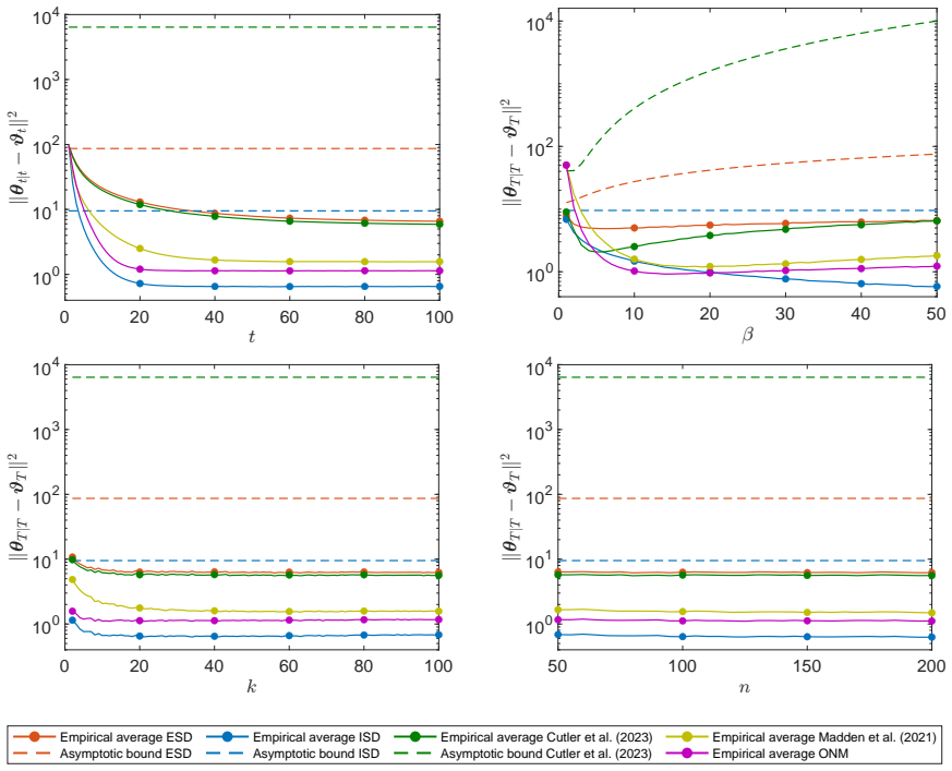
Can stochastic gradient methods track a moving target? We study the problem of tracking multidimensional time-varying parameters under noisy observations and possible model misspecification. Gradient-based filters update the time-varying parameters using the gradient of a postulated objective function. A natural filtering objective is the logarithm of the postulated observation density, which gives rise to the widely used class of score-driven filters. As in the optimization literature, these filters come in two forms: explicit filters evaluate the gradient at the predicted parameter, whereas implicit filters evaluate it at the updated parameter. For both filter types, we derive novel sufficient conditions for exponential stability of the filtered parameter path, showing that stability can be guaranteed independently of the data-generating process. Under mild additional moment conditions on the data-generating process, we also obtain finite-sample and asymptotic mean squared error bounds relative to the pseudo-true parameter path. For implicit filters, these guarantees hold under weak parameter restrictions. For explicit filters, they additionally require Lipschitz continuity of the score and a sufficiently small learning rate. Simulation studies support our theoretical findings and show that implicit gradient filters outperform explicit ones in both accuracy and stability.
Editorial analysis
A structured set of objections, weighed in public.
Referee Report
Summary. The paper studies gradient-based filters (explicit and implicit) for tracking multidimensional time-varying parameters under noisy observations and model misspecification. It derives novel sufficient conditions for exponential stability of the filtered parameter path that hold independently of the data-generating process, along with finite-sample and asymptotic MSE bounds relative to the pseudo-true path under mild moment conditions on the DGP. For implicit filters the guarantees require only weak parameter restrictions; for explicit filters they additionally require Lipschitz continuity of the score and a sufficiently small learning rate. Simulation studies are presented to support the theory.
Significance. If the stability and bound derivations hold with the claimed independence from the DGP, the results would supply useful theoretical justification for score-driven filters in misspecified environments, extending contraction-mapping ideas from optimization to filtering. The explicit/implicit distinction and the provision of both stability and error bounds are constructive contributions.
major comments (2)
- [Abstract / explicit-filter stability theorem] Abstract and statement of main stability result for explicit filters: the claim that exponential stability holds independently of the DGP requires a uniform contraction mapping. If the Lipschitz constant L(y) of the score is permitted to depend on the observation y, the one-step contraction factor of the map θ ↦ θ − η · score(θ, y) is not uniform over observation sequences; the paper must therefore clarify whether the Lipschitz condition is required to be uniform in y (with L independent of y) or only pointwise, and show how uniformity is obtained from the stated assumptions.
- [Explicit-filter stability derivation] Section deriving the explicit-filter stability (likely §3 or §4): the proof sketch that stability is independent of the DGP appears to rest on a contraction whose rate is controlled by ηL; without an explicit uniform bound on L (or a demonstration that the moment conditions already imply such a bound), the independence claim is not yet load-bearing.
minor comments (2)
- [Introduction / notation section] Notation for the pseudo-true path should be introduced earlier and used consistently when stating the MSE bounds.
- [Simulation studies] The simulation section would benefit from reporting the exact learning-rate values used and whether they satisfy the small-η condition derived in the theory.
Simulated Author's Rebuttal
We thank the referee for the careful reading and the constructive comments on the stability claims. We address the two major comments below and will revise the manuscript to improve clarity on the uniformity of the Lipschitz condition.
read point-by-point responses
-
Referee: [Abstract / explicit-filter stability theorem] Abstract and statement of main stability result for explicit filters: the claim that exponential stability holds independently of the DGP requires a uniform contraction mapping. If the Lipschitz constant L(y) of the score is permitted to depend on the observation y, the one-step contraction factor of the map θ ↦ θ − η · score(θ, y) is not uniform over observation sequences; the paper must therefore clarify whether the Lipschitz condition is required to be uniform in y (with L independent of y) or only pointwise, and show how uniformity is obtained from the stated assumptions.
Authors: We agree that the contraction must be uniform for the DGP-independence claim to hold. The manuscript assumes a uniform Lipschitz condition on the score (i.e., there exists L < ∞ independent of y such that ||score(θ, y) - score(θ', y)|| ≤ L ||θ - θ'|| for all y). This is stated in the assumptions for the explicit-filter theorem and ensures the one-step map is a uniform contraction with factor controlled by ηL. We will revise the abstract and theorem statement to explicitly note that the Lipschitz condition is uniform in y, and add a short remark in the proof section showing how this yields the claimed DGP-independent stability. revision: yes
-
Referee: [Explicit-filter stability derivation] Section deriving the explicit-filter stability (likely §3 or §4): the proof sketch that stability is independent of the DGP appears to rest on a contraction whose rate is controlled by ηL; without an explicit uniform bound on L (or a demonstration that the moment conditions already imply such a bound), the independence claim is not yet load-bearing.
Authors: The uniform bound on L is supplied directly by the Lipschitz assumption in the theorem statement for explicit filters; this assumption is part of the sufficient conditions and does not depend on the DGP. The mild moment conditions on the DGP are used only for the subsequent MSE bounds, not for establishing stability. We will revise the derivation section to explicitly isolate the contraction step, state that the rate ηL is uniform by assumption, and thereby confirm that stability holds independently of the data-generating process. revision: yes
Circularity Check
No significant circularity; derivations rest on external assumptions
full rationale
The paper's central results derive sufficient conditions for exponential stability of gradient-based filters (explicit and implicit) and associated MSE bounds relative to a pseudo-true path. These rest on stated assumptions including Lipschitz continuity of the score (for explicit filters), small learning rate, and mild moment conditions on the DGP. No quoted step reduces the claimed stability or bounds by construction to quantities fitted from the same data, nor does any load-bearing premise collapse to a self-citation chain or ansatz smuggled via prior work. The pseudo-true path is defined by the postulated model under misspecification, which is a standard external benchmark rather than a fitted input renamed as prediction. The derivation chain is therefore self-contained against the listed assumptions.
Axiom & Free-Parameter Ledger
free parameters (1)
- learning rate
axioms (3)
- domain assumption Existence of a pseudo-true parameter path under the postulated model
- domain assumption Mild moment conditions on the data-generating process
- domain assumption Lipschitz continuity of the score function
Reference graph
Works this paper leans on
-
[1]
" write newline "" before.all 'output.state := FUNCTION article output.bibitem format.authors "author" output.check author format.key output output.year.check new.block format.title "title" output.check new.block crossref missing format.jour.vol output format.article.crossref output.nonnull format.pages output if new.block note output fin.entry FUNCTION b...
-
[2]
Artemova, M., F. Blasques, J. van Brummelen, and S. J. Koopman (2022a). Score-driven models: Methodology and theory. In Oxford Research Encyclopedia of Economics and Finance . Oxford University Press
-
[3]
Artemova, M., F. Blasques, J. van Brummelen, and S. J. Koopman (2022b). Score-driven models: Methods and applications. In Oxford Research Encyclopedia of Economics and Finance . Oxford University Press
-
[4]
Bernardi, E., A. Lanconelli, C. S. Lauria, and B. T. Per c in (2024). Non trivial optimal sampling rate for estimating a L ipschitz-continuous function in presence of mean-reverting O rnstein- U hlenbeck noise. https://arxiv.org/pdf/2405.10795
- [5]
-
[6]
Blasques, F., J. van Brummelen, S. J. Koopman, and A. Lucas (2022). Maximum likelihood estimation for score-driven models. Journal of Econometrics\/ 227\/ (2), 325--346
work page 2022
-
[7]
Bottou, L., F. E. Curtis, and J. Nocedal (2018). Optimization methods for large-scale machine learning. SIAM Review\/ 60\/ (2), 223--311
work page 2018
-
[8]
Bougerol, P. (1993). Kalman filtering with random coefficients and contractions. SIAM Journal on Control and Optimization\/ 31\/ (4), 942--959
work page 1993
-
[9]
Brownlees, C. and J. Llorens-Terrazas (2024). Empirical risk minimization for time series: Nonparametric performance bounds for prediction. Journal of Econometrics\/ 244\/ (1), 105849
work page 2024
-
[10]
Caivano, M. and A. Harvey (2014). Time-series models with an EGB 2 conditional distribution. Journal of Time Series Analysis\/ 35\/ (6), 558--571
work page 2014
-
[11]
Caivano, M., A. Harvey, and A. Luati (2016). Robust time series models with trend and seasonal components. SERIEs\/ 7 , 99--120
work page 2016
-
[12]
Cao, X., J. Zhang, and H. V. Poor (2019). On the time-varying distributions of online stochastic optimization. In 2019 American Control Conference (ACC) , pp.\ 1494--1500. IEEE
work page 2019
-
[13]
Creal, D., S. J. Koopman, and A. Lucas (2013). Generalized autoregressive score models with applications. Journal of Applied Econometrics\/ 28\/ (5), 777--795
work page 2013
-
[14]
Cutler, J., D. Drusvyatskiy, and Z. Harchaoui (2023). Stochastic optimization under distributional drift. Journal of Machine Learning Research\/ 24\/ (147), 1--56
work page 2023
-
[15]
Davis, R. A., W. T. Dunsmuir, and S. B. Streett (2003). Observation-driven models for P oisson counts. Biometrika\/ 90\/ (4), 777--790
work page 2003
-
[16]
Duchi, J. C. (2018). Introductory lectures on stochastic optimization. The Mathematics of Data\/ 25 , 99--186
work page 2018
-
[17]
Durbin, J. and S. J. Koopman (1997). Monte C arlo maximum likelihood estimation for non- G aussian state space models. Biometrika\/ 84\/ (3), 669--684
work page 1997
-
[18]
Durbin, J. and S. J. Koopman (2000). Time series analysis of non- G aussian observations based on state space models from both classical and B ayesian perspectives. Journal of the Royal Statistical Society Series B: Statistical Methodology\/ 62\/ (1), 3--56
work page 2000
-
[19]
Durbin, J. and S. J. Koopman (2012). Time Series Analysis by State Space Methods , Volume 38. Oxford University Press
work page 2012
-
[20]
Fahrmeir, L. (1992). Posterior mode estimation by extended K alman filtering for multivariate dynamic generalized linear models . Journal of the American Statistical Association\/ 87\/ (418), 501--509
work page 1992
-
[21]
Gorgi, P. (2018). Integer-valued autoregressive models with survival probability driven by a stochastic recurrence equation. Journal of Time Series Analysis\/ 39\/ (2), 150--171
work page 2018
-
[22]
Gorgi, P., C. Lauria, and A. Luati (2024). On the optimality of score-driven models. Biometrika\/ 111\/ (3), 865--880
work page 2024
-
[23]
Guo, L. and L. Ljung (1995). Exponential stability of general tracking algorithms. IEEE Transactions on Automatic Control\/ 40\/ (8), 1376--1387
work page 1995
-
[24]
Harvey, A. C. (1989). Forecasting, Structural Time Series Models and the K alman Filter . Cambridge University Press
work page 1989
-
[25]
Harvey, A. C. (2013). Dynamic Models for Volatility and Heavy Tails: With Applications to Financial and Economic Time Series , Volume 52. Cambridge University Press
work page 2013
-
[26]
Harvey, A. C. (2022). Score-driven time series models. Annual Review of Statistics and Its Application\/ 9\/ (1), 321--342
work page 2022
-
[27]
Harvey, A. C. and C. Fernandes (1989). Time series models for count or qualitative observations. Journal of Business & Economic Statistics\/ 7\/ (4), 407--417
work page 1989
-
[28]
Harvey, A. C. and A. Luati (2014). Filtering with heavy tails. Journal of the American Statistical Association\/ 109\/ (507), 1112--1122
work page 2014
-
[29]
Henderson, H. V. and S. R. Searle (1981). On deriving the inverse of a sum of matrices. SIAM Review\/ 23\/ (1), 53--60
work page 1981
-
[30]
Horn, R. A. and C. R. Johnson (2012). Matrix Analysis . Cambridge University Press
work page 2012
-
[31]
Jungers, R. (2009). The Joint Spectral Radius: Theory and Applications , Volume 385. Springer
work page 2009
-
[32]
Kalman, R. E. (1960). A new approach to linear filtering and prediction problems. Journal of Basic Engineering\/ 82\/ (1), 35--45
work page 1960
-
[33]
Koopman, S. J., A. Lucas, and M. Scharth (2016). Predicting time-varying parameters with parameter-driven and observation-driven models. Review of Economics and Statistics\/ 98\/ (1), 97--110
work page 2016
-
[34]
Lambert, M., S. Bonnabel, and F. Bach (2022). The recursive variational G aussian approximation (R-VGA) . Statistics and Computing\/ 32\/ (10), 1--24
work page 2022
-
[35]
Lanconelli, A. and C. S. Lauria (2024). Maximum likelihood with a time varying parameter. Statistical Papers\/ 65\/ (4), 2555--2566
work page 2024
-
[36]
Lange, R.-J. (2024a). Bellman filtering and smoothing for state--space models. Journal of Econometrics\/ 238\/ (2), 105632
- [37]
-
[38]
Lange, R.-J., B. van Os, and D. J. van Dijk (2024). Implicit score-driven filters for time-varying parameter models. https://ssrn.com/abstract=4227958
work page 2024
-
[39]
Lehmann, E. L. and G. Casella (1998). Theory of Point Estimation . Springer
work page 1998
-
[40]
Liu, D. C. and J. Nocedal (1989). On the limited memory BFGS method for large scale optimization. Mathematical Programming\/ 45\/ (1), 503--528
work page 1989
-
[41]
Madden, L., S. Becker, and E. Dall’Anese (2021). Bounds for the tracking error of first-order online optimization methods. Journal of Optimization Theory and Applications\/ 189 , 437--457
work page 2021
-
[42]
Nemirovski, A., A. Juditsky, G. Lan, and A. Shapiro (2009). Robust stochastic approximation approach to stochastic programming. SIAM Journal on Optimization\/ 19\/ (4), 1574--1609
work page 2009
-
[43]
Nesterov, Y. (1983). A method for unconstrained convex minimization problem with the rate of convergence O (1/k^2) . Doklady AN SSSR\/ 269 , 543--547
work page 1983
-
[44]
Nesterov, Y. (2003). Introductory Lectures on Convex Optimization: A Basic Course , Volume 87. Springer
work page 2003
-
[45]
Nesterov, Y. (2018). Lectures on C onvex Optimization , Volume 137. Springer
work page 2018
-
[46]
Ollivier, Y. (2018). Online natural gradient as a K alman filter. Electronic Journal of Statistics\/ 12 , 2930--2961
work page 2018
-
[47]
Sherman, J. and W. J. Morrison (1950). Adjustment of an inverse matrix corresponding to a change in one element of a given matrix. The Annals of Mathematical Statistics\/ 21\/ (1), 124--127
work page 1950
-
[48]
Simonetto, A., E. Dall'Anese, S. Paternain, G. Leus, and G. B. Giannakis (2020). Time-varying convex optimization: Time-structured algorithms and applications. Proceedings of the IEEE\/ 108\/ (11), 2032--2048
work page 2020
-
[49]
Straumann, D. and T. Mikosch (2006). Quasi-maximum-likelihood estimation in conditionally heteroscedastic time series: A stochastic recurrence equations approach. Annals of Statistics\/ 34 , 2449--2495
work page 2006
-
[50]
Toulis, P. and E. M. Airoldi (2017). Asymptotic and finite-sample properties of estimators based on stochastic gradients. Annals of Statistics\/ 45 , 1694--1727
work page 2017
-
[51]
Wilson, C., V. V. Veeravalli, and A. Nedi \'c (2019). Adaptive sequential stochastic optimization. IEEE Transactions on Automatic Control\/ 64\/ (2), 496--509
work page 2019
discussion (0)
Sign in with ORCID, Apple, or X to comment. Anyone can read and Pith papers without signing in.