REVIEW 2 major objections 7 minor 1 cited by
On the limit of random hives with GUE boundary conditions
T0 review · 2 major / 7 minor · reviewed 2026-08-08 · deepseek-v4-flash
Pith's one-line read The paper proves that random hives with independent GUE boundary conditions converge in probability to a single continuum hive, with the pointwise limit given by a variational formula over asymptotic height functions.
desk verdict Real progress on an open limit problem; two repair-level gaps (boundary cases and a covariance bound) keep the theorem from being proven as stated. read the letter →
The pith
A machine-rendered reading of the paper's core claim, the machinery that carries it, and where it could break.
The reading
What carries the argument
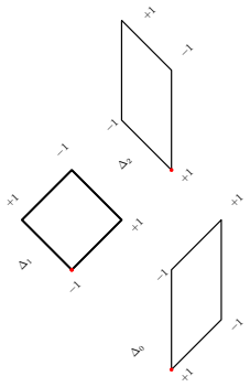
The load-bearing construction is the excavation hexagon $\mathcal{H}^n_v$ together with the octahedron recurrence: the hive value $h_n(v)$ is exactly the maximum weight of a lozenge tiling of this hexagon, with lozenge weights read from two independent GUE minor processes. The limiting variational data are the asymptotic height function pairs in $AHT^{\infty}_v$ and the functional $S_v = S_{v,\diamond}+S_{v,\Delta}+S_{v,7}$, whose bulk term integrates a surface tension $\sigma_\diamond(\rho,\partial f)$ over the hexagon. The upper bound decomposes each height function into dyadic nearly-linear patches using quantitative differentiation and controls the fluctuation of each patch with the patch-variance estimate, while the lower bound patches local optimal matchings together, so the upper and lower estimates meet at the supremum.
What would settle it
Fix an interior point $v$, simulate two independent scaled GUE minor processes up to large $n$, compute $h_n(v_n)$ as the maximum lozenge weight of the excavation hexagon via the octahedron recurrence, and compare $n^{-2}h_n(v_n)$ with the predicted supremum $\sup_{f^{\sharp} \in AHT^{\infty}_v} S_v(f^{\sharp})$. If the rescaled values do not converge, or converge to a number different from that supremum for some $v$, the central claim is wrong.
Extended reading notes
Core claim
Let $\lambda_n$ and $\mu_n$ be the eigenvalues of two independent scaled GUE matrices, and let $a_n$ be sampled from the normalized Lebesgue measure on the augmented hive polytope with those boundary data. The main theorem states that if $v_n/n \to v$, then $\lim_{n\to\infty} n^{-2} \mathbb{E}_n h_n(v_n) = \sup_{f^{\sharp} \in AHT^{\infty}_v} S_v(f^{\sharp})$, and as a corollary $n^{-2}h_n(v_n)$ converges in probability to the same value. The content is that the continuum hive is unique: the earlier subsequential limit and vanishing variance are upgraded to an exact limit, and the limiting value is the value of a specific variational problem over pairs of asymptotic height functions on the excavation hexagon.
Load-bearing premise
The upper bound requires that the maximum lozenge weight on a patch of side $m$ has variance at most $O(m^4/\log^C m)$ for every fixed $C$; the paper obtains this from a covariance decay bound for interlacing gaps of the GUE minor process quoted from an unpublished preprint, together with log-concavity. If that patch-level variance does not decay, the variational upper bound on the expected hive value fails.
Editorial extensions
If this is right
- At each fixed relative location $v$, the scaled hive value $n^{-2}h_n(v_n)$ converges in probability to the explicit number $\sup_{f^{\sharp} \in AHT^{\infty}_v} S_v(f^{\sharp})$.
- The earlier concentration result is upgraded from vanishing variance and subsequential convergence to full convergence to a single continuum hive.
- The randomized Horn problem for two independent scaled GUE matrices acquires a well-defined asymptotic law, so numerical studies can compare against a unique limit.
- The variational formula gives a computable route to the limiting value, since $S_v$ is an integral of a surface tension over the bulk plus explicit equator and hexagon terms.
Reading between the lines
- The same proof structure should yield a unique continuum limit for any ensemble of boundary data whose minor process is log-concave and has the analogous interlacing-gap covariance decay, not only GUE.
- The pointwise variational formula is strong evidence that the rate-function minimizer in the large-deviation principle for augmented hives is unique, since any minimizer must attain this supremum at every point.
- One testable extension is to compute the left-hand side numerically by direct simulation of the octahedron recurrence and compare it with an independent numerical evaluation of the variational supremum; agreement at moderate $n$ would support the formula, and disagreement would pinpoint the step to examine.
Editorial analysis
A structured set of objections, weighed in public.
Referee Report
Summary. This paper studies the augmented hives arising from the spectra of two independent scaled GUE matrices, the model that encodes the Horn probability measure for the sum of two random Hermitian matrices. The main theorem (Theorem 8.5) states that for such a hive h_n, at any vertex v_n with v_n/n → v, the normalized expectation n^{-2} E_n h_n(v_n) converges to sup_{f^♯ ∈ AHT^∞_v} S_v(f^♯), where S_v is an explicit functional of asymptotic height functions on the infinite excavation hexagon 7^∞_v; Corollary 8.6 upgrades this to convergence in probability. This would settle the uniqueness of the continuum limit left open by the author's earlier joint work with Sheffield and Tao [30], which established only subsequential convergence and vanishing variance. The proof scheme is to express the hive value as the maximum lozenge weight on an excavation hexagon, then bound this maximum from above (Sections 8.2–8.4) via a quantitative-differentiation decomposition into dyadic triangles, local variance estimates (Proposition 7.1), and the surface tension σ_⋄, and from below (Section 8.5) by explicit patching of height functions of prescribed tilt near a candidate maximizer, with separate treatment of the equator and the hexagon weight in Lemmas 8.1 and 8.2. The argument draws on fixed-index universality results for the GUE minor process quoted from Tao's preprint [40] (Theorems A.3–A.5) and on Fefferman's quantitative differentiation theorem, whose proof is reproduced in Appendix B.
Significance. If Theorem 8.5 is proved, it is a significant advance for the theory of random hives and for the randomized Horn problem: it converts the subsequential compactness of [30] into genuine convergence in probability to a single continuum limit, and it identifies the limit pointwise by a variational formula that is explicit (a supremum of integrals of the surface tension σ_⋄, itself defined from fixed-index GUE minor patches and lozenge tilings) and falsifiable by the existing simulations of [11,12]. The paper has real structural strengths: the two-sided bounds are organized around quantitative differentiation (Fefferman's theorem, proved in Appendix B), the fixed-index convergence of the GUE minor process is supported by a self-contained argument in Appendix A.4, and the surface-tension calculus of Section 11 (subadditivity, convexity, continuity, and ψ-independence) is developed in unusual detail. The paper also makes a parameter-free statement in the end: the auxiliary cutoff ψ(m) = (log m)^{-1/10} of Definition 14 is shown in Lemma 11.4 not to affect the limiting value.
major comments (2)
- [§9, Lemma 9.1, used by Prop. 7.1 and Claim 4] The bound ∥M∥_op = O(m²/log^C m) for the 4m²×4m² covariance matrix of interlacing gaps in a (2m+1)×(2m+1) patch is the load-bearing estimate for the upper bound, but the proof ('This follows from Theorem A.5, taking the parameter A in it to be sufficiently large') is ineffective. Theorem A.5 is one-dimensional and stated for fixed m: it bounds the variance of Σ_{l=1}^m a_l g̃_{i+l} for consecutive interlacing gaps along a single level of the minor process, and its right-hand side is a constant for fixed m, with no growing-m content. It therefore cannot control even a single row of the patch whose length is 2m+1, and it says nothing about covariances between gaps in different rows, which make up most of the 4m²×4m² matrix; the cross-row structure is precisely what a spectral-norm bound must control. The trivial bound on ∥M∥_op is O(m²), and without the polylogarithmic saving the variance estimate in the proof of Claim 4 (§8.4) gives O(n²) instead of o_ε(n²), so Lemma 8.7 and Lemma 8.9 are not established. The same Proposition 7.1 is used in the proof of Lemma 11.10, so the gap also propagates into Lemma 11.11, Proposition 7.5 and Proposition 8.4. I agree with the stress-test assessment: a genuinely two-dimensional covariance bound for fixed-index interlacing gaps (for example, from the determinantal kernel of the GUE minor process or from correlation decay in the bead model of [4]) must be supplied; the quoted Theorem A.5 cannot yield it.
- [Theorem 8.5, lower bound via §8.5, Lemma 8.11] Theorem 8.5 is asserted for every vertex limit v ∈ T, but the lower-bound Lemma 8.11 is proved only under the hypothesis that both trapezoids of the infinite excavation hexagon 7^∞_v contain Euclidean balls of positive radius, and this hypothesis is not stated in Theorem 8.5 or in Lemma 8.12, which appeals to Lemma 8.11 in the proof of the theorem. The hypothesis fails on the boundary of T: for v = (0, β) with 0 < β < 1 the vertices of Definition 6 give A = F and C = D, so both trapezoids collapse to line segments, and Claim 5's bound d(L_{T,ḡ}, ∂K) > cε², together with the inclusion HT^n_v(f^{♯,δ}, ε) ⊃ HT^n_v(ḡ_n, εC0) and the subsequent patching, have no geometric slack. Thus the pointwise formula is unproved for boundary points, which are included in the statement of the main theorem. The fix may be local (approximate boundary v by interior points and use continuity of both sides in v, or restrict Theorem 8.5 to the interior), but as written the theorem claims more than the proof establishes.
minor comments (7)
- [§8.4, proof of Claim 3] The choice of the constant C0 is left implicit: the line that 2^{-k}C0 → ∞ as ε → 0 is only true if C0 is taken to grow with k (e.g., C0 > 2^{2k}, which is available since 2^k < C0^{1/2} is imposed); this dependence should be stated explicitly, since in the ε → 0 asymptotics the minimal allowed C0 is astronomically large.
- [§8.4, passage from (8.6) to Lemma 8.9] The passage from the bound (8.6) for a fixed f^♯ and ε to the final display of Lemma 8.9 (limsup_{n→∞} E n^{-2} h_n(v_n) ≤ sup_{f^♯ ∈ AHT^∞_v} S_v(f^♯)) interchanges a supremum with an ε → 0 limit; this requires an explicit finite ε-covering of the compact space AHT^∞_v by tubes HT^n_v(f^♯_i, εn) with the o_ε(1) errors uniform over the finitely many centers.
- [§8.5, Lemma 8.11, last step] The last step identifies the integral against ∂f^{♯,δ} with S_{v,⋄}(f^♯) − o_ε(1), which uses δ = ε/10 → 0 together with convexity of σ_⋄(ρ,·) in the second argument (giving S_{v,⋄}(f^{♯,δ}) ≥ S_{v,⋄}(f^♯) − C_{|ρ|}δ); the text merely cites Lemma 8.3, which addresses mesh approximation rather than the δ-removal, so the step should be justified explicitly.
- [§11, proof of Lemma 11.2] The proof states that 'choosing m1 = ⌊m3/m0⌋, we see that m1m0(1 + C′ψ(m0)) = m3'; for arbitrary m3 this is not an identity, and the subadditivity inequality in Lemma 11.1 B is only stated for exact multiples with the specified border term. The rounding at both ends must be absorbed into the error terms before the argument feeds into Corollary 11.3 and Lemma 11.4.
- [§11, final paragraph of Lemma 11.4] The claimed independence of σ_⋄(ρ, a_∞) from the choice of ψ is proved in a compressed paragraph: the constants in the patching inequality are unspecified, the divisibility assumptions on m1 and m2 are not stated, and the displayed condition 'm2ψ2(m2) > m1ψ1(m1)' appears to swap the roles of ψ1 and ψ2 relative to the contradiction in (11.3). Since this paragraph establishes the parameter-freeness of the limit claimed in the main theorem, it should be expanded into a complete argument.
- [§5, Theorem 5.1 and Observation 2] The two fixed-index convergence statements are dimensionally inconsistent: the square-patch case is stated as taking values in R^{2m} with the vector 1_{2m}, while the line-segment case is stated in R^{2m+1} with 1_{2m+1}; the number of interlacing gaps in a (2m+1)×(2m+1) box should be fixed consistently, and the notation M|_{⌈ℓx⌉+2m} versus M|_{⌈ℓy⌉+l_m} should be defined with the same conventions.
- [§1.4, normalization around (1.10)–(1.11)] The normalization in §1.4 contains typos that make the scaling convention hard to verify: 'the the distribution of the eigenvalues of A + B are the pushforward', 'Cnσ−n2' (presumably C_n σ^{−n²}), and the expression 'A√σ2n' are all unclear as printed; these should be corrected.
Circularity Check
No circularity: the variational limit is computed from independent local surface-tension data, not from the hive value being predicted.
full rationale
The paper's main theorem derives a limit for n^{-2} E_n h_n(v_n) and expresses it as sup_{f^sharp in AHT^infty_v} S_v(f^sharp). The functional S_v is built from sigma_diamond, defined in Definitions 13-17 via independent GUE-minor patches and lozenge tilings, and from sigma_Delta and S_{v,7}, which are boundary and hexagon terms. None of these ingredients is defined in terms of h_n(v_n) or the target limit; the only role of the hive is the variational maximization over asymptotic height functions. The auxiliary psi(m) = (log m)^{-1/10} is chosen by hand, but Lemma 11.4 explicitly proves the limit is independent of the specific choice of psi, so this is not a fitted parameter. The proof builds on [30] and quotes Tao's unpublished Theorem A.5, but those are prior external inputs; the paper's contribution is the upper and lower bounds in Sections 8.4-8.5. The concern that Lemma 9.1 may not follow from Theorem A.5 is a correctness gap rather than circularity: it concerns an insufficient proof step, not a definitional or self-referential reduction. Consequently no step is circular.
Assumptions & free parameters
free parameters (1)
- psi(m) = (log m)^{-1/10}
assumptions (6)
- domain assumption GUE minor process converges to the Boutillier bead model in constant-size squares around bulk energies
- standard math Fefferman quantitative differentiation (Theorem 7.6)
- standard math Prekopa's theorem on log-concavity of marginal densities (Theorem 4.1)
- standard math Thurston's height function extension criteria (Propositions 10.1 and 10.2)
- domain assumption Mesoscopic CLT of Landon-Sosoe [24, Theorem 1.4] gives convergence of E[n^{-2} wt'(7_n^v)]
- domain assumption Theorem A.5 (Tao): interlacing gap statistics variance bound in fixed-index patches
Cite this review
Pith. "Pith review of On the limit of random hives with GUE boundary conditions." pith.science (2026). https://pith.science/paper/L7K6ZJAM
@misc{pith2026250206414,
  author       = {Pith},
  title        = {Pith review of: On the limit of random hives with GUE boundary conditions},
  year         = {2026},
  howpublished = {\url{https://pith.science/paper/L7K6ZJAM}},
  note         = {Machine review of arXiv:2502.06414}
}
abstract
We show that hives chosen at random with independent GUE boundary conditions on two sides, weighted by a Vandermonde factor depending on the third side (which is necessary in the context of the randomized Horn problem), when normalized so that the eigenvalues at the edge are asymptotically constant, converge in probability to a continuum hive as $n \rightarrow \infty.$ It had previously been shown in joint work with Sheffield and Tao \cite{NST} that the variance of these scaled random hives tends to $0$ and consequently, from compactness, that they converge in probability subsequentially. In the present paper, building on \cite{NST}, we prove convergence in probability to a single continuum hive, without having to pass to a subsequence. We moreover show that the value at a given point $v$ of this continuum hive equals the supremum of a certain functional acting on asymptotic height functions of lozenge tilings.
Figures


Figures from the paper (23 more)




Forward citations
Cited by 1 Pith paper
-
Hives from deformed GUE minor processes
Deformed GUE minor processes plus the octahedron recurrence yield random hives within O(n log n) KL divergence of a GUE hive law under a matching condition on the deformations.
Reference graph
Works this paper leans on
-
[30]
Sums of GUE matrices and concentration of hives from correlation decay of eigengaps
H. Narayanan, S. Sheffield, T. Tao, “Sums of GUE matrices and concentration of hives from correlation decay of eigengaps”, Probab. Theory Relat. Fields 190, 1121–1165 (2024)
work page 2024
-
[40]
On the distribution of eigenvalues of GUE and its minors at fixed index
T. Tao, “On the distribution of eigenvalues of GUE and its minors at fixed index”, preprint
-
[4]
The bead model and limit behaviors of dimer models
C. Boutillier, “The bead model and limit behaviors of dimer models”, Ann.Probab. 37,no. 1, 107–142 (2009)
work page 2009
-
[1]
The Dyson Brownian Minor Process
M. Adler, E. Nordenstam, P. Moerbeke. (2010). “The Dyson Brownian Minor Process.” Annales de l’Institut Fourier. 64. 10.5802/aif.2871
-
[2]
Y. Baryshnikov, “GUEs and queues”. Probability Theory and Related Fields, 119, 256–274 (2001)
work page 2001
-
[3]
Large deviation principles via spherical integrals
S. Belinschi, A. Guionnet, J. Huang, “Large deviation principles via spherical integrals”. Probab. Math. Phys. 3, 543–625 (2022)
work page 2022
-
[5]
A variational principle for domino tilings
H. Cohn, R. Kenyon, J. Propp, “A variational principle for domino tilings”. J. Amer. Math. Soc. 14 (2001), 297-346
work page 2001
-
[6]
From orbital measures to Littlewood-Richardson coefficients and hive polytopes
R. Coquereaux, J. B. Zuber, “From orbital measures to Littlewood-Richardson coefficients and hive polytopes”m Annales de l’Institut Henri Poincar’e (D), Combinatorics, Physics and their Interactions, European Mathematical Society, 5 (3), 339–386 (2018)
work page 2018
Show all 45 references
-
[7]
On Schur problem and Kostka numbers. In- tegrability, quantization, and geometry II
R. Coquereaux, J. B. Zuber, “On Schur problem and Kostka numbers. In- tegrability, quantization, and geometry II”, Quantum theories and algebraic geometry, 111–135, Proc. Sympos. Pure Math., 103.2 (2021)
2021
-
[8]
On Horn’s Problem and Its Volume Function
R. Coquereaux, C. McSwiggen, J. B. Zuber, “On Horn’s Problem and Its Volume Function”, Commun. Math. Phys. 376, 2409–2439 (2020)
2020
-
[9]
Wegner Estimate and Level Repulsion for Wigner Random Matrices
L. Erd˝ os, B. Schlein, H.-T. Yau, “Wegner Estimate and Level Repulsion for Wigner Random Matrices”, International Mathematics Research Notices, 2010, 436–479 (2010)
2010
-
[10]
Notes on Quantitative Differentiation
C. Fefferman, “Notes on Quantitative Differentiation”, personal communication
-
[11]
Gangopadhyay, https://github.com/aalok1993/combinatorial-hives
A. Gangopadhyay, https://github.com/aalok1993/combinatorial-hives
-
[12]
On the randomized Horn problem and the surface tension of hives
A. Gangopadhyay, H. Narayanan, “On the randomized Horn problem and the surface tension of hives.” https://arxiv.org/pdf/2410.12619.pdf (2024)
2024 arXiv
-
[13]
Lectures on Random Lozenge Tilings
V. Gorin, “Lectures on Random Lozenge Tilings” (Cambridge Studies in Advanced Mathematics). Cambridge: Cambridge University Press. (2021)
2021
-
[14]
Doubly stochastic matrices and the diagonal of a rotation matrix
A. Horn, “Doubly stochastic matrices and the diagonal of a rotation matrix”, American Journal of Mathematics 76, 620–630 (1954)
1954
-
[15]
Eigenvalues of sums of Hermitian matrices
A. Horn, “Eigenvalues of sums of Hermitian matrices”, Pacific J. Math. 12, 225–241 (1962). 54
1962
-
[16]
Eigenvalues of GUE minors. Electronic Journal of Probability
K. Johansson, and E. Nordenstam, “Eigenvalues of GUE minors. Electronic Journal of Probability”, 11, 1342-1371.(2006)
2006
-
[17]
Logarithmic bounds for isoperimetry and slices of convex sets
B. Klartag, “Logarithmic bounds for isoperimetry and slices of convex sets”, https://arxiv.org/abs/2303.14938v1 (2023)
2023 arXiv
-
[18]
Stable vector bundles and Hermitian operators
A. Klyachko, “Stable vector bundles and Hermitian operators”, Selecta Math. (N.S.), 4, 419–445 (1998)
1998
-
[19]
The honeycomb model of GLn(C) tensor products I: proof of the saturation conjecture
A. Knutson, T. Tao, “The honeycomb model of GLn(C) tensor products I: proof of the saturation conjecture”, J. Amer. Math. Soc., 12, 1055–1090 (1999)
1999
-
[20]
Honeycombs and sums of Hermitian matrices
A. Knutson, T. Tao, “Honeycombs and sums of Hermitian matrices”, Notices Amer. Math. Soc., 48 (2000)
2000
-
[21]
A Positive Proof of the Littlewood- Richardson Rule using the Octahedron Recurrence
A. Knutson, T. Tao, C. Woodward, “A Positive Proof of the Littlewood- Richardson Rule using the Octahedron Recurrence”, The Electronic Journal of Combinatorics, 11, 1 (2004)
2004
-
[22]
Schubert puzzles and integrability I: invariant trilinear forms
A. Knutson, P. Zinn-Justin, “Schubert puzzles and integrability I: invariant trilinear forms”, preprint. https://arxiv.org/abs/1706.10019 (2017)
2017 arXiv
-
[23]
Gelfand–Tsetlin Polytopes: A Story of Flow and Order Polytopes
R. Liu, K. M´ esz´ aros, A. St. Dizier, “Gelfand–Tsetlin Polytopes: A Story of Flow and Order Polytopes”, SIAM J. Discrete Math., 33(4), 2394–2415, (2019)
2019
-
[24]
B. Landon. P. Sosoe. ”Applications of mesoscopic CLTs in random matrix theory.” Ann. Appl. Probab. 30 (6) 2769 - 2795, December 2020. https://doi. org/10.1214/20-AAP1572
2020 doi
-
[25]
M. L. Mehta, Random matrices. Third edition. Pure and Applied Mathematics (Amsterdam), 142. Elsevier/Academic Press, Amsterdam, 2004
2004
-
[26]
On the role of convexity in isoperimetry, spectral gap and concen- tration
E. Milman, “On the role of convexity in isoperimetry, spectral gap and concen- tration”, Invent. Math. 177, 1–43, (2009)
2009
-
[27]
Estimating deep Littlewood-Richardson Coefficients
H. Narayanan, “Estimating deep Littlewood-Richardson Coefficients”, 26th International Conference on Formal Power Series and Algebraic Combinatorics (FPSAC 2014), 2014, Chicago, United States. 321–332
2014
-
[28]
Random discrete concave functions on an equilateral lattice with periodic Hessians
H. Narayanan, “Random discrete concave functions on an equilateral lattice with periodic Hessians.” https://arxiv.org/pdf/2005.13376.pdf (2020)
2020 arXiv
-
[29]
Large deviations for random hives and the spectrum of the sum of two random matrices
H. Narayanan, S. Sheffield, “Large deviations for random hives and the spectrum of the sum of two random matrices.” Ann. Probab. 52 (3) 1093–1152, May 2024. 55
2024
-
[31]
Why would multiplicities be log-concave?
A. Okounkov, “Why would multiplicities be log-concave?”, The Orbit Method in Geometry and Physics Progress in Mathematics 213, 329–347 (2003)
2003
-
[32]
On the largest Kronecker and Littlewood– Richardson coefficients,
I. Pak, G. Panova, D. Yeliussizov, “On the largest Kronecker and Littlewood– Richardson coefficients,” Journal of Combinatorial Theory, Series A, 165, 44–77, (2019)
2019
-
[33]
On Logarithmic Concave Measures and Functions
A. Pr´ ekopa, “On Logarithmic Concave Measures and Functions.” Acta Scien- tiarum Mathematicarum (Szeged) 34, 339–343, (1973)
1973
-
[34]
¨Uber eine Klasse von Mittelbildungen mit Anwendungen auf die Determinantentheorie
I. Schur, “ ¨Uber eine Klasse von Mittelbildungen mit Anwendungen auf die Determinantentheorie”, Sitzungsber. Berl. Math. Ges. 22, 9–20 (1923)
1923
-
[35]
Random Surfaces
S. Sheffield, “Random Surfaces”, Ast´ erisque, no. 304 (2005)
2005
-
[36]
D. E. Speyer, Perfect matchings and the octahedron recurrence, J Algebr Comb 25, 309–348 (2007)
2007
-
[37]
The asymptotic distribution of a single eigenvalue gap of a Wigner matrix
T. Tao, “The asymptotic distribution of a single eigenvalue gap of a Wigner matrix”, Probab. Theory Relat. Fields 157, 81–106 (2013)
2013
-
[38]
Random matrices: Sharp concentration of eigenvalues
T. Tao, V. Vu, “Random matrices: Sharp concentration of eigenvalues”, Random Matrices: Theory and Applications. 2, No. 03, 1350007 (2013)
2013
-
[39]
Tao, Personal Communication
T. Tao, Personal Communication
-
[41]
W. P. Thurston, Conway’s tiling groups, The American Mathematical Monthly 97, no. 8 (1990), 757 – 773
1990
-
[42]
High-Dimensional Probability: An Introduction with Appli- cations in Data Science
R. Vershynin, “High-Dimensional Probability: An Introduction with Appli- cations in Data Science” (Cambridge Series in Statistical and Probabilistic Mathematics) (2018)
2018
-
[43]
Limit laws for random matrices and free products
D. Voiculescu, “Limit laws for random matrices and free products”, Invent. Math., 104, 201–220 (1991)
1991
-
[44]
Weyl, Das asymptotische Verteilungsgesetz der Eigenwerte lineare partieller Differentialgleichungen, Math
H. Weyl, Das asymptotische Verteilungsgesetz der Eigenwerte lineare partieller Differentialgleichungen, Math. Ann. 71, 441–479, (1912). 56 A Eigenvalues of GUE A.1 Concentration of eigenvalues By Corollary 15 of Tao and Vu, [ 38], we know the following (which in fact holds for...
1912
-
[45]
As an application of the above estimates, one may now also obtain a universal law in the fixed index sense
(with a drift parameter determined by the location in the bulk). As an application of the above estimates, one may now also obtain a universal law in the fixed index sense. Define the interlacing gaps ˜gi := p N/2ρsc(γi/N)(λ′ i − λi) then we have 0 < ˜gi < gi. Informally, the ...
Reviewed August 8, 2026 · model on record in the stance chip above.
Discussion (0). Continue with ORCID to comment.