Study of the 2024 major Vela glitch at the Argentine Institute of Radioastronomy

Carlos O. Lousto; Ezequiel Zubieta; Federico Garc\'ia; Guillermo Gancio; Jorge A. Combi; Linwei Wang; Ryan Missel; Santiago del Palacio; Susana B. Araujo Furlan

REVIEW 3 major objections 5 minor 44 references

Study of the 2024 major Vela glitch at the Argentine Institute of Radioastronomy

T0 review · 3 major / 5 minor · reviewed 2026-08-08 · deepseek-v4-flash

Challenge this review Re-run · record.json Download PDF Read on arXiv ↗

Pith's one-line read The 2024 Vela glitch is measured with two exponential recovery timescales and unchanged single-pulse clustering.

desk verdict Solid, well-observed timing solution for the 2024 Vela glitch, with a real circularity problem in the claimed independent epoch estimate and a model-dependent recovery decomposition that the authors themselves flag. read the letter →

arxiv 2502.06704 v1 pith:RU7JTWHM submitted 2025-02-10 astro-ph.HE

Ezequiel Zubieta , Ryan Missel , Susana B. Araujo Furlan , Carlos O. Lousto , Federico García , Santiago del Palacio , Guillermo Gancio , Jorge A. Combi

show 1 more author

Linwei Wang

This is my paper · ORCID

classification astro-ph.HE

keywords pulsars:Velaglitchespulsartimingself-organizingmapsvariationalautoencoderradioastronomyneutronstars

verification ladder T0 review T1 audit T2 compute T3 formal

The pith

A machine-rendered reading of the paper's core claim, the machinery that carries it, and where it could break.

The reading

This paper characterises the major glitch that hit the Vela pulsar on 2024 April 29, using high-cadence radio observations from two 30 m antennas. From pulsar timing, it measures a permanent frequency jump of $\Delta\nu_g/\nu = 2.40103(5)\times 10^{-6}$, a permanent spin-down change, and two exponential recovery components with timescales of about 3 days and 17 days. Using machine-learning clustering on roughly 1.3 million single pulses taken five days before and four days after the glitch, it finds that high-amplitude pulses arrive earlier and are narrower, but that the overall pulse population shows no qualitative systematic change across the glitch. The value of the result is that a rare, well-sampled giant glitch can be compared with earlier Vela glitches to constrain how neutron star interiors respond to sudden spin-up events.

What carries the argument

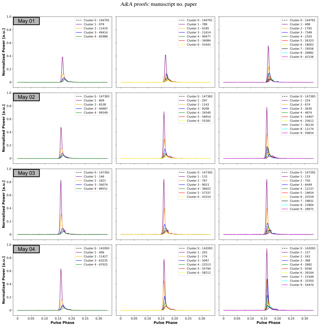
The central machinery is the glitch timing model of Eq. (2), which adds to the Taylor-expansion pulsar phase a permanent frequency jump, a permanent spin-down jump, and a sum of exponentially decaying transient frequency components, each with its own timescale $\tau_d$. The authors fit this model to the observed times of arrival with the TEMPO2 glitch plug-in, then perform a grid search over the pair $(\tau_{d1}, \tau_{d2})$ that minimises the reduced chi-squared of the residuals. For the pulse-by-pulse analysis, the machinery is a two-stage unsupervised pipeline: a variational autoencoder (a neural network that reconstructs each noisy pulse from a low-dimensional latent space) removes noise, and a self-organizing map (a competitive clustering grid) groups the denoised pulses into 4, 6, or 9 clusters per day, whose mean amplitudes, peak locations, widths, and skews are compared day by day.

What would settle it

Re-fit the same arrival times with the glitch epoch left as a free parameter and with a third, longer recovery component included; if the permanent frequency jump or the two short timescales move by more than their quoted 1$\sigma$ uncertainties, the claimed timing solution is not robust.

Watch

Extended reading notes

Core claim

The authors establish, for the 2024 April 29 Vela glitch, a complete timing solution with a relative frequency jump of $\Delta\nu_g/\nu = 2.40103(5)\times 10^{-6}$, a permanent spin-down rate change of $\Delta\dot{\nu}_p = -1.0140(8)\times 10^{-13}$ s$^{-2}$, and two transient frequency components that decay with timescales $\tau_{d1} = 17.3(3)$ d and $\tau_{d2} = 2.78(3)$ d, whose degrees of recovery sum to about 1% of the total glitch size. The reported glitch epoch, $t_g = \mathrm{MJD}\,60429.86961(4)$, agrees with the value announced in the initial alert, which the timing fit adopted as fixed. On the single-pulse side, applying a variational autoencoder to denoise individual pulses and self-organizing maps to cluster them, the authors find that the highest-amplitude pulse cluster consistently arrives earlier and is about twice as narrow as the average pulse, on all nine observed days. No qualitative systematic change appears in the clustering before versus after the glitch.

Load-bearing premise

The load-bearing premise is that the glitch epoch announced by another group ($t_g = \mathrm{MJD}\,60429.86962(4)$) is correct and that two exponential recovery terms completely describe the post-glitch relaxation; if either gives way, the fitted permanent jump and the two timescales could shift.

Editorial extensions

If this is right

The 2024 Vela glitch has a size comparable to the 2019 and 2021 giant glitches, but its recovery is dominated by two short timescales rather than a long one, suggesting that post-glitch relaxation differs between events.
Because the two recovery terms add up to only about 1% of the glitch size, most of the 2024 glitch is a permanent frequency step.
The absence of a qualitative change in single-pulse clustering around the glitch indicates that no prominent magnetospheric reconfiguration accompanied this event, in contrast to the pulse-shape changes reported for the 2016 Vela glitch.
The earlier arrival and narrower width of high-amplitude pulses, seen on all nine days, support the idea that bright pulses come from a separate emission region at a different magnetospheric altitude, and could be used for more precise pulsar timing.
The flat post-glitch residuals imply that, with the two chosen recovery components, the timing model is complete for the observed data span.

Reading between the lines

Editorial extensions of the paper, not claims the author makes directly.

[Editorial inference] If the adopted glitch epoch from the other group is even slightly biased, the two fast recovery timescales and their amplitudes could shift; an independent re-fit with the epoch left free would separate this degeneracy.
[Editorial inference] The same variational-autoencoder and self-organizing-map pipeline could be run on the 2021 Vela glitch data with the same nine-day layout, turning the qualitative 'no change' result into a quantitative comparison of how two different glitches affect the magnetosphere.
[Editorial inference] The systematic earlier arrival and narrower width of bright pulses suggests a selection of emission altitudes that could act as a high-precision timing probe; monitoring that cluster continuously across the next glitch would test whether the magnetosphere responds at the glitch epoch or only later.

Share X Bluesky LinkedIn Reddit HN

Editorial analysis

A structured set of objections, weighed in public.

Desk editor's note, referee report, and a circularity audit.

Desk Editor's Note

read the letter

You should know two things up front. First, this is a useful observational paper: it gives the best-sampled timing solution yet for the 2024 April Vela glitch, with a clean two-exponential recovery (tau_d1 = 17.3 d, tau_d2 = 2.78 d), a relative frequency jump of 2.4e-6, and a flat residual after fitting. Second, the paper overclaims its independence on the glitch epoch, and the recovery decomposition is model-dependent in a way the authors acknowledge but do not quantify.

What is genuinely new: the high-cadence timing solution itself, the two recovery timescales, and the single-pulse SOM/VAE null result around the glitch. The methods come from the same group's earlier papers, but applying them to this event with this density of TOAs is a real addition. The pulse-by-pulse null result is honestly stated: no qualitative systematic change in clustering before versus after. The comparison plot of recovery terms across Vela glitches is useful, and the paper correctly flags the known degeneracy between component number and timescales (Section 4, near Fig. 3).

Soft spots, in proportion. The circularity is real: Section 4 fixes tg to Palfreyman (2024), then the conclusions say the observations "verify and independently estimate" that same epoch. That is not independent. It may be harmless in practice — the epoch uncertainty is tiny and the phase offset absorbs some of it — but the wording needs to change. Second, the two-exponential model is chosen by grid search on the same data, and the quoted errors are conditional on that model. The stress-test concern about a third component or red noise biasing Delta_nu_p and the recovery amplitudes is legitimate; I would have liked a test adding a long timescale component or a statement that the 70-day window makes it unobservable. That said, the authors explicitly acknowledge the degeneracy, and the residuals are flat, so this is a model-uncertainty issue rather than a fatal flaw.

Minor points: no code or data release, which limits independent verification of the timing fit; the section heading "Analysis Methods: Pulse-by-pulse analysis of the 2021 Vela glitch" is a leftover typo; and the May 2 MJD in Table 2 looks garbled (6043283136500318), presumably a formatting error.

Who this is for: glitch modelers and observers who want a precise anchor for the 2024 Vela event, and anyone studying magnetospheric changes around glitches. The central timing result holds up as an empirical fit; the recovery parameters should be treated as somewhat model-dependent. I'd send this to a serious referee. A good referee will ask for the epoch language to be fixed, a model-uncertainty discussion, and ideally a data release — all addressable.

Referee Report

3 major / 5 minor

Summary. This paper reports on the 2024 April 29 glitch of the Vela pulsar using high-cadence observations from the two IAR antennas. The timing analysis yields a permanent frequency jump Delta_nu_g/nu = 2.40103(5) x 10^-6, a permanent spin-down change Delta_nu_dot_g/nu_dot = 0.107(1), and two exponential recovery terms with timescales tau_d1 = 17.3(3) d and tau_d2 = 2.78(3) d (Table 1). The single-pulse analysis of nine days around the glitch, using VAE denoising and SOM clustering, finds no qualitative systematic change in pulse morphology or clustering across the glitch, while confirming that high-amplitude pulses arrive earlier and are narrower. The paper concludes that the glitch epoch is independently verified and that the two-component recovery model is complete for the observed data.

Significance. The paper's strengths are its dense temporal coverage of a major Vela glitch, a standard and reproducible timing analysis (including EFAC/EQUAD treatment), and a clearly described null result for glitch-associated changes in single-pulse statistics. If the parameters are robust, this is one of the best-sampled Vela glitch characterizations to date and adds important data points to the recovery-timescale versus Q relation in Fig. 3. The authors also correctly cite and acknowledge the known degeneracy between the number of exponential recovery components and the fitted timescales, and they compare with their own previous analyses of the 2021 glitch.

major comments (3)

[Section 6, first paragraph] The statement 'The high cadence of our observations allowed us to verify and independently estimate the time of the glitch as tg(MJD) = 60429.86961(4), confirming the value initially reported in Palfreyman (2024)' is inconsistent with Section 4, where tg is fixed to the Palfreyman (2024) value during the fit. The uncertainty quoted in Table 1 is therefore the externally adopted uncertainty, not an independent measurement from this dataset. Please remove the word 'independently' and rephrase to state that the timing solution is consistent with the previously reported epoch.
[Section 4, Eq. (2) and Fig. 2] The grid search over tau_d1 and tau_d2 and the quoted 1-sigma to 3-sigma contours are conditional on the two-exponential model. The paper acknowledges the degeneracy between the number of components and the timescales, but it does not quantify how the presence of a third (longer) recovery component, such as the one found for the 2021 Vela glitch in Zubieta et al. (2024d), would shift Delta_nu_p, Delta_nu_d1, Delta_nu_d2, tau_d1, and tau_d2. Given the claim that the residuals are flat and the timing model is complete, please either add a fit with an additional component to bound this systematic shift, or explicitly state that the quoted uncertainties do not include model-selection uncertainty.
[Table 1, tg row] The table lists tg = 60429.86961(4) as a parameter of the timing model, but the text explains that this value was fixed from Palfreyman (2024) rather than fitted. Please clarify in the table caption or in the text that tg is an adopted external value, not a free parameter of the fit, so that readers do not mistake the quoted uncertainty for a measurement by this analysis.

minor comments (5)

[Section 5 heading] The heading reads 'Pulse-by-pulse analysis of the 2021 Vela glitch', but the analysis presented in this paper concerns the 2024 glitch; this should be corrected.
[Table 2, May 2 row] The MJD epoch for May 2 is listed as '6043283136500318', which appears to be missing a decimal point; it should likely be 60432.83136500318.
[Section 4, final timing fit] The paper does not report the reduced chi-squared or the root-mean-square residual of the final timing solution; adding one line with this value would help readers assess the fit quality.
[Section 4, TempoNest parameters] The value TNGlobalEQ = -5.64459 is given without explanation of its sign or whether it is a logarithmic quantity; please clarify.
[Equation (2)] In Eq. (2), the factor 'd' appears in the denominator of the exponential argument (t - tg)/(tau_i d); if this denotes days, it should be defined explicitly in the text to avoid confusion with a differential element.

Circularity Check

1 steps flagged · score 4.0 of 10

The claim of independently estimating the glitch epoch is circular: Section 4 adopts Palfreyman (2024)'s tg as a fixed input, and Section 6 then presents the same value as an independent verification. The central timing and single-pulse results are empirical fits, not derivations, so the circularity is partial rather than total.

fitted input called prediction [Section 4 (2024 Vela glitch characterisation, paragraph 2) and Section 6 (Conclusions and discussion, paragraph 1)]
"At this stage we also included ∆ϕ in the timing model, assuming tg = 60429.86962(4) as reported by Palfreyman (2024). ... The high cadence of our observations allowed us to verify and independently estimate the time of the glitch as, tg(MJD) = 60429.86961(4), confirming the value initially reported in Palfreyman (2024)."

The paper's own description makes Palfreyman's epoch an input to the fit: tg is adopted as 60429.86962(4) and only ∆ϕ is added to absorb the phase offset; no free fit of tg is described. The value reported in Table 1, 60429.86961(4), differs from that input only in the last digit and carries the same quoted uncertainty (4 in the last digit), so it is the adopted input, not an independent measurement. The Section 6 statement that the observations 'verify and independently estimate' the glitch epoch therefore restates the assumption as a measured result; the claimed verification reduces to the input by construction. The remaining glitch parameters are empirical fits to TOAs and are not circular, though they are model-dependent.

full rationale

The paper is largely an observational characterization: the glitch frequency jumps, spin-down change, and two exponential recovery timescales are obtained by fitting Eq. (2) to measured TOAs, and the single-pulse SOM/VAE analysis is an empirical clustering study. These central results are not derived from the inputs by construction, so they are not circular. The one genuine circularity is the treatment of the glitch epoch: Section 4 fixes tg to the value reported by Palfreyman (2024) and includes it in the timing model as an assumed parameter, yet Section 6 claims the same observations 'verify and independently estimate' that epoch. Since the fit is conditioned on that epoch, the echoed value is not an independent estimate. The paper also honestly flags the known degeneracy between the number of recovery components and their fitted timescales, citing Antonopoulou et al. (2022); that is model-dependence, not circularity. Self-citations to earlier PuMA papers (Lousto et al. 2021; Zubieta et al. 2023) supply the clustering methodology, but the application here is to new data and does not reduce to those citations. Overall, the central measurements stand on their own, while a secondary 'independent confirmation' claim is circular; hence a partial score of 4 rather than a higher score.

Assumptions & free parameters 8 free parameters · 8 assumptions · 0 invented entities

No new physical entities, forces, or conserved quantities are introduced; all quantities are measured properties of the known pulsar. The free parameters are the fitted glitch components and recovery timescales, and the axioms are the standard timing and clustering assumptions used to produce those fits.

free parameters (8)

tau_d1 (first recovery timescale) = 17.3(3) days
Recovery timescale for the first transient frequency term, determined by grid search minimizing chi2_red (Table 1, Fig. 2).
tau_d2 (second recovery timescale) = 2.78(3) days
Second recovery timescale from the same grid search; abstract rounds to ~3 days.
Delta_nu_p (permanent frequency jump) = 2.65752(3) x 10^-5 s^-1
Permanent component of the glitch frequency jump fitted to TOAs.
Delta_nu_d1 (transient frequency amplitude 1) = 1.510(4) x 10^-7 s^-1
Amplitude of the 17-day recovery component.
Delta_nu_d2 (transient frequency amplitude 2) = 1.242(3) x 10^-7 s^-1
Amplitude of the 2.78-day recovery component.
Delta_nu_dot_p (permanent spin-down jump) = -1.0140(8) x 10^-13 s^-2
Change in spin-down rate at the glitch epoch.
Delta_phi (phase offset at glitch) = 0.00676(9)
Phase offset included to absorb glitch epoch uncertainty.
Number of exponential recovery components = 2
Chosen by inspecting residuals and grid search; paper acknowledges degeneracy between component number and timescales.

assumptions (8)

standard math The pulsar's rotational phase follows a Taylor expansion in frequency and its derivatives (Eq. 1).
Standard timing model used to predict TOAs; invoked in Section 3.
domain assumption The glitch adds a permanent frequency jump plus a sum of exponentially decaying frequency increments (Eq. 2).
Functional form adopted from McCulloch et al. (1987); used to fit the glitch in Section 4.
domain assumption The glitch epoch reported by Palfreyman (2024), MJD 60429.86962(4), is correct and is used as a fixed input.
Section 4 says 'assuming tg = 60429.86962(4) as reported by Palfreyman (2024)'. This is external, not measured in this paper.
domain assumption Dispersion measure is constant at DM = 67.93(1) pc cm^-3 from the ATNF catalogue.
Used for dedispersion and folding in Sections 3 and 5; variations stated to be small (DM < 0.2 pc cm^-3).
domain assumption EFAC/EQUAD white-noise parameters from TempoNest fully describe TOA uncertainties.
Section 4 reports T NGlobalEF = 4.1283 and T NGlobalEQ = -5.64459 and uses them in the timing fit.
domain assumption Two exponential recovery terms are sufficient to model the post-glitch residuals.
Section 4 adds terms until residuals are flat; the paper cites the known degeneracy in the number of components (Antonopoulou et al. 2022).
domain assumption The VAE trained on one observation generalizes to other days without biasing reconstructed pulse shapes.
Section 5.1 and Appendix B use one VAE for all nine days; raw pulse examples are shown as a sanity check.
domain assumption Pulse amplitudes in arbitrary units, without flux calibration, are adequate for comparing pre/post-glitch distributions.
Section 5.2 notes amplitudes are arbitrary because no flux calibrator was observed; relative distributions are compared day to day.

how reviews work

0 comments

Cite this review

Pith. "Pith review of Study of the 2024 major Vela glitch at the Argentine Institute of Radioastronomy." pith.science (2026). https://pith.science/paper/RU7JTWHM

@misc{pith2026250206704,
  author       = {Pith},
  title        = {Pith review of: Study of the 2024 major Vela glitch at the Argentine Institute of Radioastronomy},
  year         = {2026},
  howpublished = {\url{https://pith.science/paper/RU7JTWHM}},
  note         = {Machine review of arXiv:2502.06704}
}

abstract

We report here on new results of the systematic monitoring of southern glitching pulsars at the Argentine Institute of Radioastronomy. In particular, we study in this work the new major glitch in the Vela pulsar (PSR J0835$-$4510) that occurred on 2024 April 29. We aim to thoroughly characterise the rotational behaviour of the Vela pulsar around its last major glitch and investigate the statistical properties of its individual pulses around the glitch. We characterise the rotational behaviour of the pulsar around the glitch through the pulsar timing technique. We measured the glitch parameters by fitting timing residuals to the data collected during the days surrounding the event. In addition, we study Vela individual pulses during the days of observation just before and after the glitch. We selected nine days of observations around the major glitch on 2024 April 29 and studied their statistical properties with the Self-Organizing Maps (SOM) technique. We used Variational AutoEncoder (VAE) reconstruction of the pulses to separate them clearly from the noise. We obtain a precise timing solution for the glitch. We find two recovery terms of $\sim 3~\mathrm{days}$ and $\sim 17~\mathrm{days}$. We find a correlation of high amplitude with narrower pulses while not finding notable qualitative systematic changes before and after the glitch.

Figures

Figures reproduced from arXiv: 2502.06704 by the authors.

**Figure 2.** Best fit of the decay time constants τd1 and τd2 for the 2024 Vela glitch. The solid line, dashed line, and dot-dashed line indicate the 1-, 2- and 3-σ confidence regions. (2023). We first obtained the pre-glitch rotational model by fitting ν, ˙ν and ¨ν to the TOAs before the glitch, keeping the value of DM = 67.93(1) pc cm−3 from the ATNF pulsar catalogue2 . We show the residuals corresponding to the pre-glitch ti… view at source ↗

**Figure 3.** Comparison of current and previous glitches decaying parameters for Vela pulsar. ble 2. Those are uninterrupted single observations with A2 antenna observations typically lasting 3.66 hours. All observations were folded with a fixed DM = 67.93(1) pc cm−3 from the ATNF catalogue3 (as we have seen very small variations during each observation, DM < 0.2 pc cm−3 ) and cleaned from radio frequency interferences using … view at source ↗

Figures from the paper (4 more)

**Figure 4.** Figure 4: Peak amplitude of single pulses distribution for observations with A2 preglitch on April 17-20,28, and post glitch on May1-5, 2024. The top yellow curve is the cumulative sum. The high cadence of our observations allowed us to verify and independently estimate the time…

**Figure 5.** Figure 5: Mean cluster reconstruction for observations with A2 before the glitch on 2024, April 17, 18, 19, 20, and 28, using 4, 6, and 9 SOM clustering. [200 (out of total 611) phase bins were taken around the mean peak (at bin 100) of each day to perform the single-pulse analy…

**Figure 6.** Figure 6: Mean cluster reconstruction for observations with A2 after the glitch on 2024, May 1, 2, 3, and 4, using 4, 6, and 9 SOM clustering. [200 (out of total 611) phase bins were taken around the mean peak (at bin 100) of each day to perform the single-pulse analysis]. ysis …

**Figure 7.** Figure 7: Peak location and magnetosphere altitude, with the corresponding error bars, for each of the pulse 4-clusters and the whole observation. Acknowledgements We especially thank Yogesh Maan for numerous beneficial discussions about the best use of RFIClean. COL gratefull…

Discussion (0). Continue with ORCID to comment.

Reference graph

Works this paper leans on

44 extracted references · 40 canonical work pages

[1]

A., Chau, H

Alpar, M. A., Chau, H. F., Cheng, K. S., & Pines, D. 1993, ApJ, 409, 345

work page 1993
[2]

Andersson, N., Glampedakis, K., Ho, W. C. G., & Espinoza, C. M. 2012, Phys. Rev. Lett., 109, 241103

work page 2012
[3]

Antonopoulou, D., Haskell, B., & Espinoza, C. M. 2022, Reports on Progress in Physics, 85, 126901 Araujo Furlan, S. B., Gancio, G., Galante, C. A., & Romero, G. E. 2023, Boletin de la Asociacion Argentina de Astronomia La Plata Argentina, 64, 304

work page 2022
[4]

D., Graber, V ., & Palfreyman, J

Ashton, G., Lasky, P. D., Graber, V ., & Palfreyman, J. 2019, Nature Astronomy, 3, 1143

work page 2019
[5]

2022, MNRAS, 510, 4049

Basu, A., Shaw, B., Antonopoulou, D., et al. 2022, MNRAS, 510, 4049

work page 2022
[6]

M., & Levin, Y

Bransgrove, A., Beloborodov, A. M., & Levin, Y . 2020, ApJ, 897, 173

work page 2020
[7]

H., Johnston, S., & Das, P

Cairns, I. H., Johnston, S., & Das, P. 2001, ApJ, 563, L65

work page 2001
[8]

2013, Phys

Chamel, N. 2013, Phys. Rev. Lett., 110, 011101

work page 2013

Show all 44 references

[9]

G., McCulloch, P

Dodson, R. G., McCulloch, P. M., & Lewis, D. R. 2002, ApJ, 564, L85

2002
[10]

M., Lyne, A

Espinoza, C. M., Lyne, A. G., Stappers, B. W., & Kramer, M. 2011, MNRAS, 414, 1679

2011
[11]

Flanagan, C. S. 1990, Nature, 345, 416

1990
[12]

O., Combi, L., et al

Gancio, G., Lousto, C. O., Combi, L., et al. 2020, A&A, 633, A84

2020
[13]

E., Astudillo, J., Saavedra, E

Gancio, G., Romero, G. E., Astudillo, J., Saavedra, E. A., & Combi, J. A. 2024, in Revista Mexicana de Astronomia y Astrofisica Conference Series, V ol. 56, Revista Mexicana de Astronomia y Astrofisica Conference Series, 131–133

2024
[14]

2018, ApJ, 865, 23 Gügercino˘glu, E

Graber, V ., Cumming, A., & Andersson, N. 2018, ApJ, 865, 23 Gügercino˘glu, E. 2017, in Journal of Physics Conference Series, V ol. 932, Jour- nal of Physics Conference Series (IOP), 012037 Gügercino˘glu, E. & Alpar, M. A. 2020, MNRAS, 496, 2506

2018
[15]

& Melatos, A

Haskell, B. & Melatos, A. 2015, International Journal of Modern Physics D, 24, 1530008

2015
[16]

Ho, W. C. G., Espinoza, C. M., Antonopoulou, D., & Andersson, N. 2015, Sci- ence Advances, 1, e1500578

2015
[17]

N., et al

Hobbs, G., Coles, W., Manchester, R. N., et al. 2012, MNRAS, 427, 2780

2012
[18]

W., van Straten, W., & Manchester, R

Hotan, A. W., van Straten, W., & Manchester, R. N. 2004, PASA, 21, 302

2004
[19]

2001, The Astrophysical Journal, 549, L101

Johnston, S., van Straten, W., Kramer, M., & Bailes, M. 2001, The Astrophysical Journal, 549, L101

2001
[20]

& Haskell, B

Khomenko, V . & Haskell, B. 2018, Publications of the Astronomical Society of Australia, 35, e020

2018
[21]

Kingma, D. P. & Welling, M. 2014, Auto-Encoding Variational Bayes

2014
[22]

1988, Self-Organized Formation of Topologically Correct Feature Maps (Cambridge, MA, USA: MIT Press), 509–521

Kohonen, T. 1988, Self-Organized Formation of Topologically Correct Feature Maps (Cambridge, MA, USA: MIT Press), 509–521

1988
[23]

P., et al

Lentati, L., Alexander, P., Hobson, M. P., et al. 2014, MNRAS, 437, 3004

2014
[24]

I., & Lattimer, J

Link, B., Epstein, R. I., & Lattimer, J. M. 1999, Phys. Rev. Lett., 83, 3362 Lopez Armengol, F. G., Lousto, C. O., del Palacio, S., et al. 2019a, The As- tronomer’s Telegram, 12482, 1 Lopez Armengol, F. G., Lousto, C. O., del Palacio, S., et al. 2019b, The As- tronomer’s Teleg...

1999
[25]

O., Missel, R., Prajapati, H., et al

Lousto, C. O., Missel, R., Prajapati, H., et al. 2021, Monthly Notices of the Royal Astronomical Society [https://academic.oup.com/mnras/advance-article-pdf/doi/10.1093/mnras/stab3287/41243307/stab3287.pdf], stab3287

2021 doi
[26]

Lyne, A. G. 1992, Philosophical Transactions of the Royal Society of London Series A, 341, 29

1992
[27]

2021, A&A, 650, A80

Maan, Y ., van Leeuwen, J., & V ohl, D. 2021, A&A, 650, A80

2021
[28]

D., Palfreyman, J

Mahida, A. D., Palfreyman, J. L., Calves, G. M., & Sett, S. 2023, Mon. Not. Roy. Astron. Soc., 524, 759

2023
[29]

Manchester, R. N. 2018, in IAU Symposium, V ol. 337, Pulsar Astrophysics the Next Fifty Years, ed. P. Weltevrede, B. B. P. Perera, L. L. Preston, & S. Sanidas, 197–202

2018
[30]

N., Hobbs, G

Manchester, R. N., Hobbs, G. B., Teoh, A., & Hobbs, M. 2005, AJ, 129, 1993

2005
[31]

1987, Australian Journal of Physics, 40, 725

Mcculloch, P., Klekociuk, A., Hamilton, P., & Royle, G. 1987, Australian Journal of Physics, 40, 725

1987
[32]

Montoli, A., Antonelli, M., & Pizzochero, P. M. 2020, MNRAS, 492, 4837

2020
[33]

2024, The Astronomer’s Telegram, 16615, 1

Palfreyman, J. 2024, The Astronomer’s Telegram, 16615, 1

2024
[34]

M., Hotan, A., Ellingsen, S., & van Straten, W

Palfreyman, J., Dickey, J. M., Hotan, A., Ellingsen, S., & van Straten, W. 2018, Nature, 556, 219

2018
[35]

L., Dickey, J

Palfreyman, J. L., Dickey, J. M., Ellingsen, S. P., Jones, I. R., & Hotan, A. W. 2016, ApJ, 820, 64

2016
[36]

H., Teukolsky, S

Press, W. H., Teukolsky, S. A., Vetterling, W. T., & Flannery, B. P. 1992, Numer- ical recipes in C. The art of scientific computing (IOP Publishing)

1992
[37]

& Manchester, R

Radhakrishnan, V . & Manchester, R. N. 1969, Nature, 222, 228

1969
[38]

2011, PRESTO: PulsaR Exploration and Search TOolkit

Ransom, S. 2011, PRESTO: PulsaR Exploration and Search TOolkit

2011
[39]

2018, PRESTO - Pulsar Exploration and Search Toolkit

Ransom, S. 2018, PRESTO - Pulsar Exploration and Search Toolkit

2018
[40]

Reichley, P. E. & Downs, G. S. 1969, Nature, 222, 229

1969
[41]

2021, The Astronomer’s Tele- gram, 14806, 1

Sosa-Fiscella, V ., Zubieta, E., del Palacio, S., et al. 2021, The Astronomer’s Tele- gram, 14806, 1

2021
[42]

Taylor, J. H. 1992, Philosophical Transactions of the Royal Society of London, 341, 117

1992
[43]

2024e, arXiv e-prints, arXiv:2412.17766

Zubieta, E., García, F., del Palacio, S., et al. 2024e, arXiv e-prints, arXiv:2412.17766

arXiv
[44]

Zubieta, E. et al. 2023, Mon. Not. Roy. Astron. Soc., 521, 4504 Article number, page 9 of 13 A&A proofs: manuscript no. paper Appendix A: Tables of SOM Clustering Here we include the numerical information in tabular form about the clustering analysis summarised in Fig. 5-6. Th...

2021

Pith tools

Reviewed August 8, 2026 · model on record in the stance chip above.

[1] [1]

A., Chau, H

Alpar, M. A., Chau, H. F., Cheng, K. S., & Pines, D. 1993, ApJ, 409, 345

work page 1993

[2] [2]

Andersson, N., Glampedakis, K., Ho, W. C. G., & Espinoza, C. M. 2012, Phys. Rev. Lett., 109, 241103

work page 2012

[3] [3]

Antonopoulou, D., Haskell, B., & Espinoza, C. M. 2022, Reports on Progress in Physics, 85, 126901 Araujo Furlan, S. B., Gancio, G., Galante, C. A., & Romero, G. E. 2023, Boletin de la Asociacion Argentina de Astronomia La Plata Argentina, 64, 304

work page 2022

[4] [4]

D., Graber, V ., & Palfreyman, J

Ashton, G., Lasky, P. D., Graber, V ., & Palfreyman, J. 2019, Nature Astronomy, 3, 1143

work page 2019

[5] [5]

2022, MNRAS, 510, 4049

Basu, A., Shaw, B., Antonopoulou, D., et al. 2022, MNRAS, 510, 4049

work page 2022

[6] [6]

M., & Levin, Y

Bransgrove, A., Beloborodov, A. M., & Levin, Y . 2020, ApJ, 897, 173

work page 2020

[7] [7]

H., Johnston, S., & Das, P

Cairns, I. H., Johnston, S., & Das, P. 2001, ApJ, 563, L65

work page 2001

[8] [8]

2013, Phys

Chamel, N. 2013, Phys. Rev. Lett., 110, 011101

work page 2013