Musical Score Following using Statistical Inference

Josephine Cowley

REVIEW 4 major objections 5 minor 56 references

Musical Score Following using Statistical Inference

T0 review · 4 major / 5 minor · reviewed 2026-08-09 · deepseek-v4-flash

Challenge this review Re-run · record.json Download PDF Read on arXiv ↗ Review JSON

Pith's one-line read A Gaussian-process note-likelihood model plus a duration-aware HMM tracks a live performance through a score in real time.

desk verdict A genuine first proof-of-concept of GP-based score following, undermined by a purely qualitative evaluation that does not quantify the headline success claim. read the letter →

arxiv 2502.10426 v1 pith:HXRNXBNB submitted 2025-02-06 eess.AS cs.SDeess.SP

Josephine Cowley This is my paper · ORCID

classification eess.AScs.SDeess.SP

keywords scorefollowingGaussianprocessspectralmixturekernelhiddenMarkovmodelViterbialgorithmmusicinformationretrievalreal-timeaudiopitchinference

verification ladder T0 review T1 audit T2 compute T3 formal

The pith

A machine-rendered reading of the paper's core claim, the machinery that carries it, and where it could break.

The reading

Musical score following is the real-time mapping of a performance to a location in the score. This report argues that Gaussian processes (GPs) can provide the statistical core of that mapping: a GP with a spectral-mixture kernel scores every candidate set of notes for an audioframe, and a duration-aware hidden Markov model turns those frame scores into a running estimate of score position. The claim is that this two-stage pipeline follows simple keyboard pieces and, without retraining, solo flute, oboe, and violin recordings, including passages with heavy rubato. If true, this is a first proof of concept that GP audio models are efficient and flexible enough for online music information retrieval tasks like automatic page turning and accompaniment.

What carries the argument

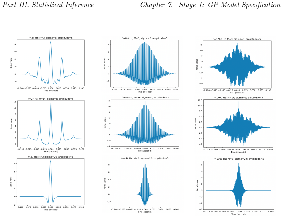
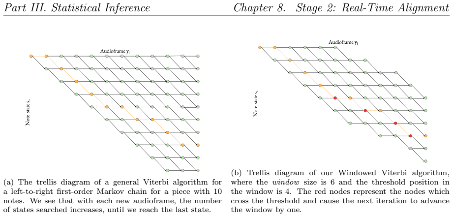
The load-bearing object is the spectral-mixture covariance function $$k(\tau) = $e^{{-2\pi^2\sigma_f^2\tau^2}}$\sum_{q=1}^Q w_q \sum_{m=1}^M E_m \cos(2\pi m f_q b_{m,f_q}\tau),$$ obtained as the inverse Fourier transform of a mixture of Gaussians placed at the harmonic frequencies of each candidate note. Here $f_q$ encodes the candidate note, $E_m = 1/(1+T m^v)$ sets the harmonic envelope, $b_{m,f_q} = \sqrt{1+B_{f_q}m^2}$ corrects inharmonicity, and $\sigma_f$ governs the tolerated frequency spread. The log marginal likelihood of an audioframe under this kernel is computed with a Cholesky factorization and used as the HMM's emission probability. The HMM is left-to-right with a geometric state-duration model whose expected state length is estimated from MIDI durations and a moving-average tempo conversion; a windowed Viterbi search then keeps the maximum a posteriori path computable online.

What would settle it

Perform a controlled comparison of the same piano piece recorded with no pedal, moderate pedal, and heavy pedal, manually annotating the true score position for every audioframe. If per-frame accuracy is near-perfect without pedal but drops sharply under heavy pedal—as the paper's own results suggest—the claim that the GP likelihood generalizes across normal playing conditions is falsified.

Watch

Extended reading notes

Core claim

The central claim is that a stationary spectral-mixture Gaussian process, whose covariance function is constructed from the expected harmonic power spectrum of pitched notes, produces a sharply peaked log marginal likelihood at the true fundamental frequency of a piano audioframe, and that this likelihood can serve as the emission model of an HMM for real-time score alignment. The report demonstrates this on a monophonic keyboard piece where the follower never deviated by more than a semiquaver, on a two-part Minuet where it recovered from a missed left-hand note, on a four-part hymn arranged for keyboard, and on solo flute, oboe, and violin recordings despite heavy rubato. It also reports degradation under excessive sustain pedal, repeated notes, and heavy ornamentation, and identifies these as the main limitations.

Load-bearing premise

The hand-tuned note-likelihood model, chosen on isolated piano frames, keeps giving reliable likelihoods for real performances on other instruments, at other tempi, and when the sustain pedal changes the sound.

Editorial extensions

If this is right

Because the same piano-tuned likelihood followed wind and string instruments, one GP acoustic model can serve as the front end of a real-time score follower without per-instrument retraining.
Automatic page turning and computer-aided accompaniment become practical with only a MIDI score and a microphone, since the pipeline runs in real time on audioframes of about 18 ms.
The windowed Viterbi restricts the search to a sliding window, so runtime scales with window size rather than with the total length of the piece.
Rubato and local tempo changes are absorbed by the duration model's moving-average tempo conversion, but only as long as the performer substantially follows the score; ornaments and omitted notes can still break alignment.

Reading between the lines

Editorial extensions of the paper, not claims the author makes directly.

Because the same piano-trained kernel followed flute, oboe, and violin, one can reasonably test the frame-level LML as a general pitch-observation model for instrument identification or source separation; that would be an extension beyond the paper's scope.
The failures under heavy sustain pedal and repeated notes both strain the left-to-right, no-backtracking HMM assumption, so replacing the transition model with a multi-resolution or jump-capable HMM would show whether those failures are structural or merely tuning artifacts.
The hyperparameters were chosen from LML plots on isolated piano frames, so a sensitivity sweep over those values on sustained-pedal recordings would reveal how much of the reported success depends on the particular tuning rather than on the GP framework itself.

Share X Bluesky LinkedIn Reddit HN

Signed reviews

No signed human review yet.

Editorial analysis

A structured set of objections, weighed in public.

Desk editor's note, referee report, and a circularity audit.

Desk Editor's Note

read the letter

This is an MEng thesis posted to arXiv, and it reads like one: carefully written, honest about limitations, but the central claim "we have achieved successful score following" (Sec 11.1) is supported mainly by prose descriptions of screen recordings. The stress-test note gets this right. If you are looking for a quantitative demonstration that a GP+HMM follower tracks score position accurately, this paper does not provide it. What it does provide is a genuinely new combination: a Spectral Mixture GP whose kernel is designed to model harmonic spectra with inharmonicity correction, used to produce per-frame note likelihoods that feed a duration-aware HMM with a windowed Viterbi decoder. I am not aware of prior GP-based score following, and the engineering is real: the author discusses covariance precomputation, Cholesky-based LML, multiprocessing queues, and an open-source rendering UI. The code appears to be available on GitHub, which helps reproducibility.

The paper's strengths: the GP model is physically motivated; hyperparameters like M, sigma_f, T, v are tied to observable spectral structure; the limitation sections (8.6, 10.1) openly discuss sustain-pedal failures, repeated notes, and ornamentation. That honesty is worth crediting. The author also correctly notes that score-following evaluation is not standardized, which justifies some qualitative assessment.

The soft spots are real and load-bearing. First, the evaluation is self-assessment: Section 8.6 says "visual inspection (and some manual time-mapping)" and Chapter 10 gives adjectives ("impressive", "highly accurate") rather than alignment-error numbers. No per-note or per-frame accuracy, no latency measurements, no baseline comparison. Second, the hyperparameters were explicitly selected in Section 7.4 to make LML peak at true fundamental frequencies. That is acceptable for a proof of concept, but it means the note-inference stage is fitted to the intended outcome, and the claim that the model generalizes across instruments is only supported anecdotally. Third, the scope is narrow: the HMM assumes the performer starts at the beginning and makes no significant deviations, and the author essentially avoids heavy sustain pedal in tests. These limitations are acknowledged, but they undercut the abstract's unqualified success claim.

Overall: a promising, clearly written proof of concept that deserves to be seen by reviewers, but only after quantitative evaluation is added. I would accept it for peer review with major revision. For a reader working on GP-based MIR or score following, it's worth a look; for anyone wanting a reliable follower, not yet.

Referee Report

4 major / 5 minor

Summary. The manuscript proposes a two-stage score-following system for solo piano (and, in tests, other monophonic instruments). In Stage 1, a Gaussian Process with a Spectral Mixture covariance kernel is used to compute a log marginal likelihood (LML) for each candidate note/chord state from 800–2000-sample audioframes; hyperparameters are selected so that the LML peaks at the true fundamental frequencies. In Stage 2, these LMLs are used as emission probabilities in a left-to-right HMM with a geometric state-duration model, and an approximate online 'Windowed' Viterbi algorithm tracks the most likely score position. The paper reports qualitative results on six recordings (piano, flute, oboe, violin, and a cello-piano duet) and claims successful score following, including on instruments the GP model was not designed for.

Significance. If the central claim were supported by quantitative evidence, the paper would be a useful proof-of-concept: it applies GP/Spectral-Mixture kernels to online score following, provides a stable Cholesky-based LML implementation, and contributes a modular open-source system with a real-time renderer. The cross-instrument demonstrations are intriguing and suggest the GP model may generalize beyond its piano tuning data. However, the evaluation is entirely qualitative and self-assessed; no alignment-error metrics, latency measurements, baselines, or ablation studies are reported. The scientific claim of 'successful score following' is therefore not yet established, and the paper currently reads as a detailed engineering report rather than a validated research contribution.

major comments (4)

[§10 and §8.6] The headline claim of 'successful score following' is not supported by the reported evaluation. Section 8.6 states that results were analysed by 'visual inspection (and some manual time-mapping)', and Chapter 10 presents only prose descriptions of screen recordings (e.g., 'impressive', 'highly accurate', 'primarily achieves its goal') with no quantitative alignment error, no per-note or per-frame accuracy, no latency figures, and no comparison with any baseline score follower (e.g., DTW or an HMM with standard spectral features). Since score position has a ground truth (score events versus recorded audio), objective metrics are feasible. Section 10.1 itself concedes that in the Schumann duet the follower 'rarely positions the marker on exactly the right state/note' and that repeated notes or ornaments cause it to get lost. As it stands, the central claim in the abstract and in Section 11.1 is not established.
[§7.4] The GP emission model is tuned to the intended output. The hyperparameters (M = 9, sigma_f = 0.005, T = 0.465, v = 2.37, and the per-key inharmonicity dictionary B) were selected by inspecting LML-versus-frequency plots to ensure that the LML peaks at the true fundamental frequencies for isolated piano frames (§7.4). These LMLs are then used directly as HMM emission probabilities (§8.3). No train/test split or cross-validation is described, so the piano results may partly reflect fitting to the tuning data rather than generalization. The cross-instrument results mitigate this concern, but they are only qualitative. Please add a held-out evaluation and a sensitivity analysis (e.g., varying sigma_f and M) to show that alignment performance does not depend on precisely tuned values.
[§10 (Syrinx and Schumann tests)] The abstract highlights a 'duration-dependent HMM', but two of the most successful non-piano tests were run with state_duration disabled. Section 10 states that for Syrinx 'we disabled the state_duration mode' because the local-tempo assumption failed, and for the Schumann duet state_duration was also turned off. The paper does not specify what transition model was used in these runs, nor does it provide an ablation quantifying the contribution of the duration model when it is enabled. This makes it impossible to attribute the reported performance to the two-stage GP+HMM design rather than to a simpler HMM with a flat transition model. Please report the fallback transition model and include an ablation with and without state_duration on the same pieces.
[§9.3 and §11.1] The 'real-time' claim is not quantified. The system is described as having 'low latency and no buffering' (§11.1), but no frame processing time, end-to-end delay, or CPU usage is measured. Real-time score following requires a hard bound on per-frame computation; the qualitative statement that the algorithm 'runs in real-time, at least for short recordings' (§8.6) is insufficient. Please report measured per-frame inference time (e.g., versus the 800-sample frame length and hop length) under the actual multiprocessing architecture, including worst-case behaviour.

minor comments (5)

[§8.5.2, Algorithm 1] The algorithm adds transition probabilities T^d_{k,k} and T^d_{k-1,k} directly to log-likelihoods LML(yn|sn = k). If these T^d values are probabilities, they should be log-transformed before addition; please clarify the notation.
[§7.3.2] The spectral-envelope expression Em = 1/(1+T m^v) is ambiguous: the exponent v is introduced without a clear symbol for the harmonic index m, and the subscript m on Em is inconsistently used elsewhere. Please define all symbols explicitly in one place.
[§9.3.1] There is a typo in the heading: 'Score Preprocesor' should be 'Score Preprocessor'.
[§11.1] The statement that successful score following 'by definition' also means that GPs are capable of score alignment is not a definitional consequence; online tracking does not automatically imply that an offline alignment algorithm works. The claim should be softened or justified.
[§6.2.1 and §10] Section 6.2.1 declares 'subjective evaluation of trained musicians' as the primary benchmark, but no structured expert evaluation is reported; the descriptions in Chapter 10 appear to be the author's self-assessment. Please either report a formal expert study or clearly label the results as informal demo observations.

Circularity Check

1 steps flagged · score 5.0 of 10

Stage 1's frequency-prediction evidence reuses the LML-peak criterion used to tune the GP; the full score-following tests are independent but qualitative.

fitted input called prediction [Section 7.4 ('σf: Inverse Length Scale') and Section 7.5 ('Results and Discussion')]
"Then, for audioframes of varying f, we plotted LML vs. fundamental frequency for a logarithmic range of σf centring around 0.01, examining the graphs for prominent global maxima at the true fundamental frequency... Finally, we settled for σf = 0.005. ... The key result from this chapter is shown in Figure 7.9. The largest peak occurs at the true fundamental frequency of the audioframe, as indicated by the red dashed line."

The hyperparameter σf (together with M, T, v, and B) is selected by directly inspecting LML-versus-frequency plots for 'prominent global maxima at the true fundamental frequency'. The chapter's headline evidence of accurate pitch prediction is then the same kind of LML plot, and the text describes no held-out split. For any audioframe used in that selection, the reported peak is a restatement of the fitting objective rather than an independent prediction. The full-system HMM tests in Sections 8.6 and 10 use complete separate recordings, so the central score-following claim retains independent content; the circularity is therefore limited to Stage 1's single-frame inference evidence.

full rationale

The GP kernel hyperparameters are fitted to typical piano audioframes by visual and numerical optimisation of LML plots, which is normal model fitting. The circular element arises only where the same fitted objective—an LML peak at the true fundamental—is then presented as the key successful result of Stage 1 without any stated train/test separation. The two-stage follower is additionally tested on complete pieces (Bach, Solfeggietto, Syrinx, etc.), which were not the isolated tuning frames; those tests provide independent, though purely qualitative, evidence for the score-following claim. There is no load-bearing self-citation, no imported uniqueness theorem, and no renamed benchmark. The main weakness of the paper is the absence of quantitative alignment-error metrics, which is an evidence gap rather than a circularity. The score of 5 reflects the Stage 1 fit/prediction conflation while acknowledging that the downstream HMM evaluation has independent content.

Assumptions & free parameters 6 free parameters · 7 assumptions · 0 invented entities

The central results rest on several hand-selected hyperparameters and modeling assumptions. The paper tunes the kernel to make the target behavior (LML peak at the true note) explicit, so the contribution is a proof of concept rather than a parameter-free derivation.

free parameters (6)

M (number of harmonics) = 9
Selected from LML vs. M plots; LML plateaus past about 9 harmonics (Figure 7.6).
sigma_f (kernel inverse length scale) = 0.005
Chosen to produce prominent LML peaks at the true fundamental frequency (Figure 7.7).
T and v (spectral envelope parameters) = T = 0.465, v = 2.37
Jointly optimized using scipy.optimize on typical audioframes (Section 7.4).
B (per-key inharmonicity constants) = 88 per-key values, not listed in the paper
Constructed via L-BFGS for the specific piano used; values are not reported.
sigma_n (noise variance) = user-set, varied between 0.0001 and 10
Left to the user at runtime; changed in experiments to mitigate sustain pedal effects.
Windowed Viterbi window size and threshold = ell = 6, phi = 4 in Figure 8.4
Example values shown; no systematic selection or sensitivity analysis is reported.

assumptions (7)

domain assumption The Spectral Mixture GP is a valid generative model for audioframes (Section 7.3).
The covariance function is derived from the observed power spectrum, but no posterior predictive check or goodness-of-fit is reported.
domain assumption Audioframes are stationary (Section 7.2).
The GP assumes a stationary kernel; note decay and transients violate this mildly, which the authors acknowledge as a simplification.
domain assumption The log marginal likelihood serves directly as the HMM emission probability (Sections 7.3.4 and 8.3).
No calibration or normalization of the LML across states is described; using an unnormalized LML as a likelihood can bias the Viterbi path.
domain assumption The HMM is left-to-right with only self- and advance-transitions (Section 8.3.1).
The system cannot handle mistakes that skip notes or go backwards, which the authors state as an assumption.
domain assumption The performer starts at the beginning and makes no significant deviations (Section 8.1).
This scopes the proof of concept to performances that stay on the score.
domain assumption Spectral envelope model Em = 1/(1 + T m^v) from [23].
An empirical model for harmonic amplitudes, cited but not independently validated in this paper.
domain assumption Inharmonicity correction fm,q = m fq sqrt(1 + B_f m^2) from [17].
A standard piano model used to shift harmonic frequencies; B values are fitted per key.

how reviews work

0 comments

Cite this review

Pith. "Pith review of Musical Score Following using Statistical Inference." pith.science (2026). https://pith.science/paper/HXRNXBNB

@misc{pith2026250210426,
  author       = {Pith},
  title        = {Pith review of: Musical Score Following using Statistical Inference},
  year         = {2026},
  howpublished = {\url{https://pith.science/paper/HXRNXBNB}},
  note         = {Machine review of arXiv:2502.10426}
}

read the original abstract

Musical score following is the real-time mapping of a performance to corresponding locations in a musical score. Score following can be used in a variety of applications including automatic page turning and real-time accompaniment. This report presents a novel approach for score following motivated by Wilson and Adams's 2013 paper, which introduces Spectral Mixture (SM) kernels for Gaussian Process (GP) regression. Since the SM kernel is derived from a Mixture of Gaussians in the frequency domain, it is particularly suitable for modelling the superposed power spectra of musical notes, in which energy is concentrated at multiples of the fundamental frequency of each note. Our score follower begins by using a GP to statistically infer the musical notes played during 800-sample 'audioframes' (~18 ms) of solo piano music. These predictions are then used in a duration-dependent Hidden Markov Model to predict the most likely score positions in real time. Our two-stage approach achieves successful score following not only on four-part hymns arranged for keyboard, but also on pieces for the violin, oboe, and flute. This showcases the powerful and flexible nature of GPs for statistical inference on musical audio signals. Given the success of this project, we contribute to the literature a first proof of concept of the application of GPs in score following, and more broadly, in online Music Information Retrieval (MIR) tasks. This project also contributes a working score follower product that renders score position in real time using an adapted open-source user interface. Areas for future work include improving accuracy on repeated notes and during heavy use of sustain pedal, adapting to minor deviations from the score, and modelling multi-instrument works.

Figures

Figures reproduced from arXiv: 2502.10426 by the authors.

**Figure 1.1.** Illustration of score following: positions (blue) in the musical score are mapped to locations [PITH_FULL_IMAGE:figures/full_fig_p009_1_1.png] view at source ↗

**Figure 2.** [PITH_FULL_IMAGE:figures/full_fig_p011_2.png] view at source ↗

Figures from the paper (37 more)

**Figure 2.1.** Figure 2.1: Examples from [23] of different instruments’ temporal envelopes (top) and spectrograms (bottom). Spectrograms represent the time-varying magnitude spectra—i.e. the modulus of the shorttime Fourier transform. Audio data and images are from the RWCP Instrument samples…

**Figure 1.** Figure 1 [PITH_FULL_IMAGE:figures/full_fig_p013_1.png]

**Figure 5.** Figure 5 [PITH_FULL_IMAGE:figures/full_fig_p019_5.png]

**Figure 5.1.** Figure 5.1: Here we present random samples drawn from three different GP models which have dif [PITH_FULL_IMAGE:figures/full_fig_p020_5_1.png]

**Figure 6.** Figure 6 [PITH_FULL_IMAGE:figures/full_fig_p021_6.png]

**Figure 6.1.** Figure 6.1: Diagram depicting the high-level score follower framework, where numbers represent the steps [PITH_FULL_IMAGE:figures/full_fig_p021_6_1.png]

**Figure 7.** Figure 7: b [PITH_FULL_IMAGE:figures/full_fig_p024_7.png]

**Figure 7.1.** Figure 7.1: Two time-amplitude graphs from a recording of the note A4 ( [PITH_FULL_IMAGE:figures/full_fig_p024_7_1.png]

**Figure 7.2.** Figure 7.2: Examples of audio frequency spectra in a 2000-sample audioframe of a single A4 ( [PITH_FULL_IMAGE:figures/full_fig_p024_7_2.png]

**Figure 7.3.** Figure 7.3: Example of inharmonicity effects and how the multiplicative factor [PITH_FULL_IMAGE:figures/full_fig_p025_7_3.png]

**Figure 7.** Figure 7: a [PITH_FULL_IMAGE:figures/full_fig_p026_7.png]

**Figure 7.4.** Figure 7.4: Illustration of the covariance function defined in [PITH_FULL_IMAGE:figures/full_fig_p027_7_4.png]

**Figure 7.5.** Figure 7.5: Three randomly drawn GP samples using the covariance function defined in [PITH_FULL_IMAGE:figures/full_fig_p027_7_5.png]

**Figure 7.** Figure 7 [PITH_FULL_IMAGE:figures/full_fig_p029_7.png]

**Figure 7.6.** Figure 7.6: Graphs of LML against M for two piano notes 2 octaves apart. T and v: Spectral Envelope T and v determine the overall shape of the spectral envelope as the relative weights of the m-th harmonic is defined by Em = 1 1+Tmv . To obtain a starting point for joint optimis…

**Figure 7.** Figure 7 [PITH_FULL_IMAGE:figures/full_fig_p030_7.png]

**Figure 7.7.** Figure 7.7: LML vs. frequency for various σf (red is high, green is low) for notes over two octaves apart. w: Relative Weights of Note Sources In audioframes containing multiple notes, the relative energies of those notes will almost always be non-uniform. This is due to physica…

**Figure 7.** Figure 7: a [PITH_FULL_IMAGE:figures/full_fig_p031_7.png]

**Figure 7.8.** Figure 7.8: Graphs of G3, D4 interval, exhibiting large relative amplitude difference (D4 is much louder) [PITH_FULL_IMAGE:figures/full_fig_p031_7_8.png]

**Figure 7.** Figure 7 [PITH_FULL_IMAGE:figures/full_fig_p032_7.png]

**Figure 7.9.** Figure 7.9: Final result illustrating the variation in LML for varying frequency of a single F4 piano note [PITH_FULL_IMAGE:figures/full_fig_p032_7_9.png]

**Figure 8.** Figure 8 [PITH_FULL_IMAGE:figures/full_fig_p034_8.png]

**Figure 8.2.** Figure 8.2: Illustration of the left-to-right first [PITH_FULL_IMAGE:figures/full_fig_p034_8_2.png]

**Figure 8.** Figure 8 [PITH_FULL_IMAGE:figures/full_fig_p037_8.png]

**Figure 8.3.** Figure 8.3: Trellis diagram of the set of possible paths during the first five audioframes of the Viterbi [PITH_FULL_IMAGE:figures/full_fig_p037_8_3.png]

**Figure 8.4.** Figure 8.4: Two trellis diagrams illustrating the general and Windowed Viterbi algorithm. [PITH_FULL_IMAGE:figures/full_fig_p038_8_4.png]

**Figure 8.** Figure 8 [PITH_FULL_IMAGE:figures/full_fig_p038_8.png]

**Figure 8.** Figure 8: c [PITH_FULL_IMAGE:figures/full_fig_p039_8.png]

**Figure 8.5.** Figure 8.5: We show results from three different recordings of Bach’s [PITH_FULL_IMAGE:figures/full_fig_p039_8_5.png]

**Figure 9.** Figure 9 [PITH_FULL_IMAGE:figures/full_fig_p041_9.png]

**Figure 9.1.** Figure 9.1: Abstracted system architecture diagram displaying inputs in grey, the 4 main components of [PITH_FULL_IMAGE:figures/full_fig_p041_9_1.png]

**Figure 9.2.** Figure 9.2: System architecture diagram representing the Score Preprocessor with inputs in grey, processes [PITH_FULL_IMAGE:figures/full_fig_p041_9_2.png]

**Figure 9.3.** Figure 9.3: System architecture diagram representing the Audio Preprocessor with inputs in grey, pro [PITH_FULL_IMAGE:figures/full_fig_p042_9_3.png]

**Figure 9.4.** Figure 9.4: System architecture diagram representing the Follower and Backend processes with processes [PITH_FULL_IMAGE:figures/full_fig_p042_9_4.png]

**Figure 9.5.** Figure 9.5: System architecture diagram representing the overall score follower running in Pre-recorded [PITH_FULL_IMAGE:figures/full_fig_p043_9_5.png]

**Figure 9.** Figure 9 [PITH_FULL_IMAGE:figures/full_fig_p043_9.png]

**Figure 9.6.** Figure 9.6: Screenshot of the score renderer user interface which displays a score (here we show a keyboard [PITH_FULL_IMAGE:figures/full_fig_p043_9_6.png]

Discussion (0). Continue with ORCID to comment.

Reference graph

Works this paper leans on

56 extracted references · 52 canonical work pages

[1]

Sparse Gaussian Process Audio Source Separation Using Spectrum Priors in the Time-domain

Pablo Alvarado, Mauricio A. Alvarez, and Dan Stowell. “Sparse Gaussian Process Audio Source Separation Using Spectrum Priors in the Time-domain”. In: ICASSP 2019 - 2019 IEEE Interna- tional Conference on Acoustics, Speech and Signal Processing (ICASSP) (May 2019), pp. 995–999. doi: 10.1109/ICASSP.2019.8683287. (Visited on 12/24/2023)

work page arXiv 2019
[2]

Gaussian processes for music audio modelling and content analysis

Pablo A Alvarado and Dan Stowell. “Gaussian processes for music audio modelling and content analysis”. In: arXiv (Cornell University) (Sept. 2016). doi: 10.1109/mlsp.2016.7738836. (Visited on 01/02/2024)

work page arXiv 2016
[3]

A multi-resolution hidden Markov model using class-specific features

Paul M. Baggenstoss. “A multi-resolution hidden Markov model using class-specific features”. In: 2008 16th European Signal Processing Conference . 2008, pp. 1–5

work page 2008
[4]

Artificial Intelligence and Music: Implementing an Interactive Computer Performer

Bridget Baird, Donald Blevins, and Noel Zahler. “Artificial Intelligence and Music: Implementing an Interactive Computer Performer”. In: Computer Music Journal 17 (1993), p. 73. doi: 10.2307/ 3680871. (Visited on 07/25/2019)

work page 1993
[5]

The artificially intelligent computer performer: The second generation

Bridget Baird, Donald Blevins, and Noel Zahler. “The artificially intelligent computer performer: The second generation”. In:Interface 19 (Jan. 1990), pp. 197–204.doi: 10.1080/09298219008570566. (Visited on 12/15/2019)

work page doi:10.1080/09298219008570566 1990
[6]

Real-Time Computer Accompaniment of Keyboard Per- formances

Joshua Bloch and Roger B Dannenberg. “Real-Time Computer Accompaniment of Keyboard Per- formances”. In: ICMC 1985 (Jan. 1985). (Visited on 01/02/2024)

work page 1985
[7]

Short-time Viterbi for online HMM decoding : evaluation on a real-time phone recognition task

Julien Bloit and Xavier Rodet. Short-time Viterbi for online HMM decoding : evaluation on a real-time phone recognition task . ICASSP, Apr. 2008. url: https : / / web . archive . org / web / 20170924195402id_/https://hal.archives-ouvertes.fr/hal-01161222/document (visited on 05/08/2024)

work page 2008
[8]

Decoding HMMs using the k best paths: algorithms and applications

Daniel G. Brown and Daniil Golod. “Decoding HMMs using the k best paths: algorithms and applications”. In: BMC Bioinformatics 11 (2010), S28–S28. url: https://api.semanticscholar. org/CorpusID:671009

work page 2010

Show all 56 references

[9]

Score-Performance Matching using HMMs

Pedro Cano, `Alex Loscos, and Jordi Bonada. “Score-Performance Matching using HMMs”. In: International Computer Music Conference 1999 (Jan. 1999). (Visited on 01/02/2024)

1999
[11]

An effective method for audio-to-score alignment using onsets and modified constant Q spectra

Chunta Chen and Jyh-Shing Roger Jang. “An effective method for audio-to-score alignment using onsets and modified constant Q spectra”. In: Multimedia Tools and Applications 78 (July 2018), pp. 2017–2044. doi: 10.1007/s11042-018-6349-y . (Visited on 03/13/2023)

2018 doi
[12]

YIN, a fundamental frequency estimator for speech and music

Alain de Cheveign´ e and Hideki Kawahara. “YIN, a fundamental frequency estimator for speech and music.” In: The Journal of the Acoustical Society of America 111 4 (2002), pp. 1917–30. url: https://api.semanticscholar.org/CorpusID:1607434

2002
[13]

Improvement of Observation Modeling for Score Following

Arshia Cont. “Improvement of Observation Modeling for Score Following”. In: (Jan. 2004). url: https : / / www . researchgate . net / publication / 250796139 _ Improvement _ of _ Observation _ Modeling_for_Score_Following

2004
[14]

A Monophonic Pitch-Tracking Algorithm Based on Waveform Periodicity Determinations Using Landmark Points

David Cooper and Kia C. Ng. “A Monophonic Pitch-Tracking Algorithm Based on Waveform Periodicity Determinations Using Landmark Points”. In: Computer Music Journal 20.3 (1996), pp. 70–78. issn: 01489267, 15315169. url: http://www.jstor.org/stable/3680825 (visited on 05/22/2024)

1996
[15]

An On-Line Algorithm for Real-Time Accompaniment

Roger Dannenberg. “An On-Line Algorithm for Real-Time Accompaniment”. In: Computer Music Journal 10 2 (Jan. 1984), pp. 10–32

1984
[16]

New Techniques for Enhanced Quality of Computer Accompaniment

Roger B Dannenberg and Hirofumi Mukaino. “New Techniques for Enhanced Quality of Computer Accompaniment”. In: International Computer Music Conference 1988 (Jan. 1988). (Visited on 01/02/2024)

1988
[17]

Bayesian analysis of polyphonic western tonal music

Manuel Davy, Simon Godsill, and J´ erˆ ome Idier. “Bayesian analysis of polyphonic western tonal music”. In: The Journal of the Acoustical Society of America 119.4 (Apr. 2006), pp. 2498–2517. issn: 0001-4966. doi: 10.1121/1.2168548. url: https://doi.org/10.1121/1.2168548

2006 doi
[18]

Inference in Hidden Markov Models with Explicit State Duration Distributions

Michael Dewar, Chris Wiggins, and Frank Wood. “Inference in Hidden Markov Models with Explicit State Duration Distributions”. In: IEEE Signal Processing Letters 19.4 (Apr. 2012), pp. 235–238. issn: 1558-2361. doi: 10.1109/lsp.2012.2184795 . url: http://dx.doi.org/10.1109/LSP. ...

2012
[19]

MATCH: A Music Alignment Tool Chest

Simon Dixon and Gerhard Widmer. “MATCH: A Music Alignment Tool Chest”. In: International Symposium/Conference on Music Information Retrieval 2005 (Jan. 2005), pp. 492–497. (Visited on 01/02/2024)

2005
[20]

LEARNING SPECTRAL FILTERS FOR SINGLE-AND MULTI-LABEL CLAS- SIFICATION OF MUSICAL INSTRUMENTS

Patrick Donnelly. LEARNING SPECTRAL FILTERS FOR SINGLE-AND MULTI-LABEL CLAS- SIFICATION OF MUSICAL INSTRUMENTS . Aug. 2015. url: https://www.cs.montana.edu/ sheppard/theses/donnelly-phd.pdf (visited on 05/11/2024)

2015
[21]

Towards Score Following In Sheet Music Images

Matthias Dorfer, Andreas Arzt, and Gerhard Widmer. “Towards Score Following In Sheet Music Images.” In: International Symposium/Conference on Music Information Retrieval (Jan. 2016), pp. 789–795. (Visited on 01/02/2024)

2016
[22]

The viterbi algorithm

G.D. Forney. “The viterbi algorithm”. In: Proceedings of the IEEE 61.3 (1973), pp. 268–278. doi: 10.1109/PROC.1973.9030

1973
[23]

Bayesian statistical methods for audio and music processing

Simon Godsill et al. “Bayesian statistical methods for audio and music processing”. In: ed. by Anthony O’Hagan and Mike West. The Oxford Handbook of Applied Bayesian Analysis. Oxford University Press, 2010. Chap. 25, pp. 711–745

2010
[24]

Parallel Processing Techniques for Estimating Pitch Periods of Speech in the Time Domain

B. Gold and L. Rabiner. “Parallel Processing Techniques for Estimating Pitch Periods of Speech in the Time Domain”. In: The Journal of the Acoustical Society of America 46.2B (Aug. 1969), pp. 442–448. issn: 0001-4966. doi: 10.1121/1.1911709 . eprint: https://pubs.aip.org/asa/ ...

1969 doi
[25]

Real-Time Music Following in Score Sheet Images via Multi-Resolution Prediction

Florian Henkel and Gerhard Widmer. “Real-Time Music Following in Score Sheet Images via Multi-Resolution Prediction”. In: Frontiers in Computer Science 3 (2021). issn: 2624-9898. doi: 10.3389/fcomp.2021.718340. url: https://www.frontiersin.org/articles/10.3389/fcomp. 2021.718340

2021
[26]

Discrete time techniques for time delay estimation

G. Jacovitti and G. Scarano. “Discrete time techniques for time delay estimation”. In: IEEE Trans- actions on Signal Processing 41.2 (1993), pp. 525–533. doi: 10.1109/78.193195

1993 doi
[27]

Survey on Extraction of Sinusoids in Stationary Sounds

Florian Keiler and Sylvain Marchand. “Survey on Extraction of Sinusoids in Stationary Sounds”. In: (Nov. 2002)

2002
[28]

Musical Score Following and Audio Alignment

Lin Hao Lee. “Musical Score Following and Audio Alignment”. In: ArXiv abs/2205.03247 (2022). url: https://api.semanticscholar.org/CorpusID:248562558

2022 arXiv
[29]

Gaussian Processes for Underdetermined Source Separation

Antoine Liutkus, Roland Badeau, and G¨ ael Richard. “Gaussian Processes for Underdetermined Source Separation”. In: IEEE Transactions on Signal Processing 59 (July 2011), pp. 3155–3167. doi: 10.1109/tsp.2011.2119315. (Visited on 01/28/2020)

2011
[30]

Mel Frequency Cepstral Coefficients for Music Modeling

Beth Logan. “Mel Frequency Cepstral Coefficients for Music Modeling”. In: International Society for Music Information Retrieval Conference . 2000. url: https://api.semanticscholar.org/ CorpusID:17454278

2000
[31]

Fast, Accurate Pitch Detection Tools for Music Analysis

Philip McLeod. “Fast, Accurate Pitch Detection Tools for Music Analysis”. In: 2008. url: https: //api.semanticscholar.org/CorpusID:63088633

2008
[32]

A smarter way to find pitch

Philip McLeod and Geoff Wyvill. “A smarter way to find pitch”. In: Jan. 2005

2005
[33]

Musical String Inharmonicity

Chris Murray and Scott Whitfield. Musical String Inharmonicity. 2021. url: https://publicwebuploads. uwec.edu/documents/Musical-string-inharmonicity-Chris-Murray.pdf

2021
[34]

Real-Time Audio-to-Score Align- ment of Music Performances Containing Errors and Arbitrary Repeats and Skips

Tomohiko Nakamura, Eita Nakamura, and Shigeki Sagayama. “Real-Time Audio-to-Score Align- ment of Music Performances Containing Errors and Arbitrary Repeats and Skips”. In: IEEE/ACM Transactions on Audio, Speech, and Language Processing 24.2 (2016), pp. 329–339. doi: 10.1109/ T...

2016
[35]

Cepstrum Pitch Determination

A. Michael Noll. “Cepstrum Pitch Determination”. In: The Journal of the Acoustical Society of America 41.2 (Feb. 1967), pp. 293–309. issn: 0001-4966. doi: 10.1121/1.1910339. eprint: https: //pubs.aip.org/asa/jasa/article- pdf/41/2/293/18757858/293\_1\_online.pdf . url: https:/...

1967 doi
[36]

Adaptive Score-Following System by Integrat- ing Gaze Information

Kaede Noto, Yoshinari Takegawa, and Keiji Hirata. “Adaptive Score-Following System by Integrat- ing Gaze Information”. In: 16th Sound and Music Computing Conference (SMC2019) 16 (2019). url: https : / / www . smc2019 . uma . es / articles / S6 / S6 _ 04 _ SMC2019 _ paper . pdf...

2019
[37]

Alignment of Monophonic and Polyphonic Music to a Score

Nicola Orio, Diemo Schwarz, and Ircam Pompidou. “Alignment of Monophonic and Polyphonic Music to a Score”. In: HAL (Le Centre pour la Communication Scientifique Directe) (Sept. 2001). (Visited on 01/02/2024)

2001
[38]

On the use of autocorrelation analysis for pitch detection

Lawrence R. Rabiner. “On the use of autocorrelation analysis for pitch detection”. In: IEEE Trans- actions on Acoustics, Speech, and Signal Processing 25 (1977), pp. 24–33. url: https : / / api . semanticscholar.org/CorpusID:17947159. 43 Part V. Discussion Bibliography

1977
[39]

Automatic segmentation of acoustic musical signals using hidden Markov models

C. Raphael. “Automatic segmentation of acoustic musical signals using hidden Markov models”. In: IEEE Transactions on Pattern Analysis and Machine Intelligence 21 (Apr. 1999), pp. 360–370. doi: 10.1109/34.761266. (Visited on 12/25/2019)

1999 doi
[40]

Aligning music audio with symbolic scores using a hybrid graphical model

Christopher Raphael. “Aligning music audio with symbolic scores using a hybrid graphical model”. In: Machine Learning 65 (May 2006), pp. 389–409. doi: 10.1007/s10994-006-8415-3 . (Visited on 03/07/2021)

2006 doi
[41]

Gaussian Processes for Machine Learning

C Rasmussen and C Williams. “Gaussian Processes for Machine Learning”. In: Adaptive Computa- tion and Machine Learning Series. (2006). url: https://gaussianprocess.org/gpml/chapters/ RW.pdf

2006
[42]

Gaussian processes (3/3) - exploring kernels

Peter Roelants. Gaussian processes (3/3) - exploring kernels . peterroelants.github.io, Jan. 2019. url: https : / / peterroelants . github . io / posts / gaussian - process - kernels/(visited on 05/19/2024)

2019
[43]

Ryry: A Real-Time Score-Following Au- tomatic Accompaniment Playback System Capable of Real Performances with Errors, Repeats and Jumps

Shinji Sako, Ry¯ oichi Yamamoto, and Tadashi Kitamura. “Ryry: A Real-Time Score-Following Au- tomatic Accompaniment Playback System Capable of Real Performances with Errors, Repeats and Jumps”. In: Lecture Notes in Computer Science (Jan. 2014), pp. 134–145. doi: 10.1007/978-3-...

2014 doi
[44]

Marginalised Gaussian Processes with Nested Sampling

Fergus Simpson, Vidhi Lalchand, and Carl Edward Rasmussen. “Marginalised Gaussian Processes with Nested Sampling”. In: arXiv (Cornell University) (Oct. 2020). doi: 10.48550/arxiv.2010. 16344. (Visited on 01/08/2024)

2020 doi
[45]

Rastislav ˇSrˆ amek.The on-line Viterbi algorithm . 2007. url: http://www.dcs.fmph.uniba.sk/ diplomovky/obhajene/getfile.php/main.pdf?id=143&fid=289&type=application%2Fpdf (visited on 05/08/2024)

2007
[46]

Design and implementation of a robust pitch de- tector based on a parallel processing technique

R.A. Sukkar, J.L. LoCicero, and J.W. Picone. “Design and implementation of a robust pitch de- tector based on a parallel processing technique”. In: IEEE Journal on Selected Areas in Commu- nications 6.2 (1988), pp. 441–451. doi: 10.1109/49.619

1988 doi
[47]

A wavelet-based pitch detector for musical signals

“A wavelet-based pitch detector for musical signals”. English. In: Proceedings of 2nd COST-G6 Workshop on Digital Audio Effects (DAFx99) . Ed. by J Tro and M Larsson. Norwegian University of Science and Technology, 1999, pp. 101–104

1999
[48]

Time-Frequency Analysis as Probabilistic Inference

Richard E Turner and Maneesh Sahani. “Time-Frequency Analysis as Probabilistic Inference”. In: IEEE Transactions on Signal Processing 62 (Dec. 2014), pp. 6171–6183. doi: 10.1109/tsp.2014. 2362100. (Visited on 11/29/2023)

2014 doi
[49]

Score Following by Temporal Pattern

Jason D. Vantomme. “Score Following by Temporal Pattern”. In: Computer Music Journal 19 (1995), p. 50. doi: 10.2307/3680654. (Visited on 01/21/2019)

1995 doi
[50]

The Synthetic Performer in The Context of Live Performance

Barry Vercoe. “The Synthetic Performer in The Context of Live Performance”. In: International Computer Music Conference 1984 (Jan. 1984), pp. 199–200. (Visited on 01/02/2024)

1984
[51]

Chromagram visualization of the singing voice

Gregory H. Wakefield. “Chromagram visualization of the singing voice”. In: Proc. Models and Analysis of Vocal Emissions for Biomedical Applications (MA VEBA 1999) . 1999, pp. 24–29

1999
[52]

Gaussian Process Modelling for Audio Signals

William Wilkinson. Gaussian Process Modelling for Audio Signals . Queen Mary University of Lon- don, 2019. url: https://theses.eurasip.org/media/theses/documents/william-wilkinson- gaussian-process-modelling-for-audio-signals.pdf

2019
[53]

Gaussian Process Kernels for Pattern Discov- ery and Extrapolation

Andrew Gordon Wilson and Ryan Prescott Adams. “Gaussian Process Kernels for Pattern Discov- ery and Extrapolation”. In: arXiv:1302.4245 [cs, stat] (Dec. 2013). arXiv: 1302.4245 [stat.ML]

2013 arXiv
[54]

Robust on-line algorithm for real-time audio-to-score alignment based on a delayed decision and anticipation framework

Ry¯ oichi Yamamoto, Shinji Sako, and Tadashi Kitamura. “Robust on-line algorithm for real-time audio-to-score alignment based on a delayed decision and anticipation framework”. In: IEEE In- ternational Conference on Acoustics, Speech and Signal Processing (May 2013). doi: 10.1...

2013
[55]

Infinite Kernel Linear Prediction for Joint Estimation of Spectral Envelope and Fundamental Frequency

Kazuyoshi Yoshii and Masataka Goto. “Infinite Kernel Linear Prediction for Joint Estimation of Spectral Envelope and Fundamental Frequency”. In: IEEE International Conference on Acoustics, Speech and Signal Processing (ICASSP) (May 2013), pp. 463–467. doi: 10.1109/ICASSP.2013. 6637690

2013 doi
[56]

Beyond NMF: Time-Domain Audio Source Separation without Phase Reconstruction

Kazuyoshi Yoshii et al. “Beyond NMF: Time-Domain Audio Source Separation without Phase Reconstruction”. In: International Society for Music Information Retrieval Conference . Semantic Scholar. 2013. url: https://www.semanticscholar.org/paper/Beyond-NMF%3A-Time-Domain- Audio-So...

2013
[57]

Constant-Q signal analysis and synthesis

J. Youngberg and S. Boll. “Constant-Q signal analysis and synthesis”. In: ICASSP ’78. IEEE International Conference on Acoustics, Speech, and Signal Processing . Vol. 3. 1978, pp. 375–378. doi: 10.1109/ICASSP.1978.1170547. 44

1978

Pith tools

Reviewed August 9, 2026 · model on record in the stance chip above.

[1] [1]

Sparse Gaussian Process Audio Source Separation Using Spectrum Priors in the Time-domain

Pablo Alvarado, Mauricio A. Alvarez, and Dan Stowell. “Sparse Gaussian Process Audio Source Separation Using Spectrum Priors in the Time-domain”. In: ICASSP 2019 - 2019 IEEE Interna- tional Conference on Acoustics, Speech and Signal Processing (ICASSP) (May 2019), pp. 995–999. doi: 10.1109/ICASSP.2019.8683287. (Visited on 12/24/2023)

work page arXiv 2019

[2] [2]

Gaussian processes for music audio modelling and content analysis

Pablo A Alvarado and Dan Stowell. “Gaussian processes for music audio modelling and content analysis”. In: arXiv (Cornell University) (Sept. 2016). doi: 10.1109/mlsp.2016.7738836. (Visited on 01/02/2024)

work page arXiv 2016

[3] [3]

A multi-resolution hidden Markov model using class-specific features

Paul M. Baggenstoss. “A multi-resolution hidden Markov model using class-specific features”. In: 2008 16th European Signal Processing Conference . 2008, pp. 1–5

work page 2008

[4] [4]

Artificial Intelligence and Music: Implementing an Interactive Computer Performer

Bridget Baird, Donald Blevins, and Noel Zahler. “Artificial Intelligence and Music: Implementing an Interactive Computer Performer”. In: Computer Music Journal 17 (1993), p. 73. doi: 10.2307/ 3680871. (Visited on 07/25/2019)

work page 1993

[5] [5]

The artificially intelligent computer performer: The second generation

Bridget Baird, Donald Blevins, and Noel Zahler. “The artificially intelligent computer performer: The second generation”. In:Interface 19 (Jan. 1990), pp. 197–204.doi: 10.1080/09298219008570566. (Visited on 12/15/2019)

work page doi:10.1080/09298219008570566 1990

[6] [6]

Real-Time Computer Accompaniment of Keyboard Per- formances

Joshua Bloch and Roger B Dannenberg. “Real-Time Computer Accompaniment of Keyboard Per- formances”. In: ICMC 1985 (Jan. 1985). (Visited on 01/02/2024)

work page 1985

[7] [7]

Short-time Viterbi for online HMM decoding : evaluation on a real-time phone recognition task

Julien Bloit and Xavier Rodet. Short-time Viterbi for online HMM decoding : evaluation on a real-time phone recognition task . ICASSP, Apr. 2008. url: https : / / web . archive . org / web / 20170924195402id_/https://hal.archives-ouvertes.fr/hal-01161222/document (visited on 05/08/2024)

work page 2008

[8] [8]

Decoding HMMs using the k best paths: algorithms and applications

Daniel G. Brown and Daniil Golod. “Decoding HMMs using the k best paths: algorithms and applications”. In: BMC Bioinformatics 11 (2010), S28–S28. url: https://api.semanticscholar. org/CorpusID:671009

work page 2010