Single-Shot Matrix-Matrix Multiplication Optical Tensor Processor for Deep Learning
Pith reviewed 2026-05-22 22:13 UTC · model grok-4.3
The pith
A spatial-wavelength-temporal hyper-multiplexed architecture performs three-dimensional matrix-matrix multiplication in one optical time step.
A machine-rendered reading of the paper's core claim, the machinery that carries it, and where it could break.
Core claim
In a single time step, a three-dimensional matrix-matrix multiplication optical tensor processor is demonstrated using a spatial-wavelength-temporal hyper-multiplexed architecture that supports high computing parallelism and remains feasible for large-scale implementation, enabling acceleration of CNNs and DNNs at ultra-low optical energy of 20 attojoules per MAC with 96.4 percent classification accuracy on 292616 parameters.
What carries the argument
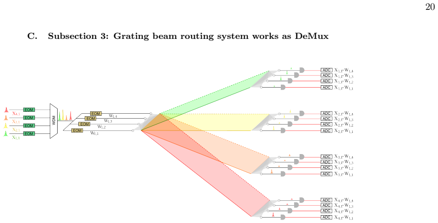
The spatial-wavelength-temporal hyper-multiplexed ONN processor architecture that encodes and processes high-dimensional data across space, spectrum, and time to perform parallel matrix multiplications.
If this is right
- CNNs and DNNs can be accelerated directly through parallel optical matrix multiplication.
- Image recognition runs at 96.4 percent accuracy using 292616 optical weights.
- Energy consumption reaches 20 attojoules per multiply-accumulate operation.
- Broad spectral and spatial bandwidths become available for larger demonstrations.
Where Pith is reading between the lines
- If the single-shot property holds at scale, inference latency could drop to the physical propagation time of light through the device.
- The approach may extend to other tensor contractions beyond matrix multiplication by reusing the same multiplexing dimensions.
- Hybrid systems could combine this optical front end with electronic backpropagation for end-to-end training at reduced energy cost.
Load-bearing premise
The hyper-multiplexed design avoids the scaling roadblocks that limited earlier high-parallelism optical neural networks when built at large size.
What would settle it
A working demonstration of the same architecture at substantially higher parameter count or dimensionality while preserving the reported energy per MAC and accuracy would support the scalability claim; inability to maintain performance at larger scales would refute it.
Figures


read the original abstract
The ever-increasing data demand craves advancements in high-speed and energy-efficient computing hardware. Analog optical neural network (ONN) processors have emerged as a promising solution, offering benefits in bandwidth and energy consumption. However, existing ONN processors exhibit limited computational parallelism, and while certain architectures achieve high parallelism, they encounter serious scaling roadblocks for large-scale implementation. This restricts the throughput, latency, and energy efficiency advantages of ONN processors. Here, we introduce a spatial-wavelength-temporal hyper-multiplexed ONN processor that supports high data dimensionality, high computing parallelism and is feasible for large-scale implementation, and in a single time step, a three-dimensional matrix-matrix multiplication (MMM) optical tensor processor is demonstrated. Our hardware accelerates convolutional neural networks (CNNs) and deep neural networks (DNNs) through parallel matrix multiplication. We demonstrate benchmark image recognition using a CNN and a subsequently fully connected DNN in the optical domain. The network works with 292,616 weight parameters under ultra-low optical energy of 20 attojoules (aJ) per multiply and accumulate (MAC) at 96.4% classification accuracy. The system supports broad spectral and spatial bandwidths and is capable for large-scale demonstration, paving the way for highly efficient large-scale optical computing for next-generation deep learning.
Editorial analysis
A structured set of objections, weighed in public.
Referee Report
Summary. The manuscript introduces a spatial-wavelength-temporal hyper-multiplexed optical neural network processor that performs three-dimensional matrix-matrix multiplication in a single time step. It reports acceleration of CNNs and DNNs for image recognition using 292616 weight parameters at 20 aJ/MAC optical energy and 96.4% classification accuracy, claiming feasibility for large-scale implementation unlike prior high-parallelism ONN designs.
Significance. If the experimental demonstration and scaling claims hold, the work would represent a notable advance in analog optical computing hardware by enabling high-dimensionality, single-shot tensor operations with ultra-low energy per MAC while addressing parallelism scaling barriers.
major comments (2)
- [Abstract] Abstract: The central claim of single-shot 3D MMM with 292616 weights at 96.4% accuracy requires that inter-channel crosstalk, spectral overlap, and insertion loss remain low enough to preserve effective MAC precision. No number of wavelength or spatial modes is stated, nor is any measured fidelity or error-rate data versus channel count supplied, leaving the scaling assumption for the hyper-multiplexed architecture unsupported.
- [Abstract] Abstract: The 20 aJ/MAC figure and 96.4% accuracy are presented as experimental results, yet the text supplies neither experimental methods, error bars, raw data, nor verification details for these quantities, preventing evaluation of the hardware claim.
Simulated Author's Rebuttal
We thank the referee for their comments and the opportunity to clarify aspects of our work. We respond point-by-point to the major comments below.
read point-by-point responses
-
Referee: [Abstract] Abstract: The central claim of single-shot 3D MMM with 292616 weights at 96.4% accuracy requires that inter-channel crosstalk, spectral overlap, and insertion loss remain low enough to preserve effective MAC precision. No number of wavelength or spatial modes is stated, nor is any measured fidelity or error-rate data versus channel count supplied, leaving the scaling assumption for the hyper-multiplexed architecture unsupported.
Authors: The abstract summarizes the demonstrated single-shot 3D MMM but does not enumerate the specific wavelength and spatial mode counts or include channel-count-dependent fidelity metrics. The full manuscript provides these details in the architecture description and experimental characterization sections, where measured crosstalk, spectral overlap, and insertion loss values are reported for the implemented channel count and shown to support the observed MAC precision. We will revise the abstract to state the number of modes employed and note that fidelity data versus channel count appear in the main text. revision: yes
-
Referee: [Abstract] Abstract: The 20 aJ/MAC figure and 96.4% accuracy are presented as experimental results, yet the text supplies neither experimental methods, error bars, raw data, nor verification details for these quantities, preventing evaluation of the hardware claim.
Authors: The 20 aJ/MAC and 96.4% accuracy values are obtained from the experimental demonstration described in the manuscript. The methods section, supplementary information, and figure captions supply the measurement procedures, verification approach, and any associated uncertainty quantification. The abstract condenses these results; we will revise it to explicitly reference the supporting experimental details in the main text. revision: yes
Circularity Check
No circularity: experimental hardware demonstration with no derivation chain
full rationale
The paper reports an experimental demonstration of a spatial-wavelength-temporal hyper-multiplexed optical neural network processor performing single-shot 3D matrix-matrix multiplication. Central claims rest on measured classification accuracy (96.4%), energy per MAC (20 aJ), and parameter count (292616) from hardware benchmarks on CNN+DNN tasks. No mathematical derivation, fitted parameters renamed as predictions, or self-citation load-bearing uniqueness theorems are present in the provided text. The architecture description and performance metrics are independent experimental results, not reductions to their own inputs by construction.
Axiom & Free-Parameter Ledger
Reference graph
Works this paper leans on
- [1]
-
[2]
A. Vaswani, N. Shazeer, N. Parmar, J. Uszkoreit, L. Jones, A. N. Gomez, Ł. Kaiser, and I. Polosukhin, Advances in neural information processing systems30 (2017)
work page 2017
-
[3]
A. Krizhevsky, I. Sutskever, and G. E. Hinton, inAdvances in Neural Information Processing Systems, Vol. 25, edited by F. Pereira, C. Burges, L. Bottou, and K. Weinberger (Curran Associates, Inc., 2012)
work page 2012
-
[4]
K. He, X. Zhang, S. Ren, and J. Sun, inProceedings of the IEEE Conference on Computer Vision and Pattern Recognition (CVPR) (2016)
work page 2016
-
[5]
I. H. Sarker, Deep learning: A comprehensive overview on techniques, taxonomy, applications and research directions (2021)
work page 2021
-
[6]
W. He, J. Li, X. Kong, and L. Deng, Communications Engineering3, 10.1038/s44172-024-00303-3 (2024)
- [7]
-
[8]
T. Ching, D. S. Himmelstein, B. K. Beaulieu-Jones, A. A. Kalinin, B. T. Do, G. P. Way, E. Ferrero, P. M. Agapow, M. Zietz, M. M. Hoffman, W. Xie, G. L. Rosen, B. J. Lengerich, J. Israeli, J. Lanchantin, S. Woloszynek, A. E. Carpenter, A. Shrikumar, J. Xu, E. M. Cofer, C. A. Lavender, S. C. Turaga, A. M. Alexandari, Z. Lu, D. J. Harris, D. Decaprio, Y. Qi,...
- [9]
-
[10]
Integrated silicon photonics: Harnessing the data explosion (2011)
work page 2011
- [11]
-
[12]
A. Yazdanbakhsh, K. Seshadri, B. Akin, J. Laudon, and R. Narayanaswami, arXiv preprint arXiv:2102.10423 (2021). 34
- [13]
- [14]
-
[15]
C. Wang, L. Gong, Q. Yu, X. Li, Y. Xie, and X. Zhou, IEEE Transactions on Computer-Aided Design of Integrated Circuits and Systems36, 513 (2017)
work page 2017
-
[16]
S. W. Keckler, W. J. Dally, B. Khailany, M. Garland, and D. Glasco, IEEE Micro31, 7 (2011)
work page 2011
- [17]
-
[18]
A. Ankit, I. E. Hajj, S. R. Chalamalasetti, G. Ndu, M. Foltin, R. S. Williams, P. Faraboschi, W.-m. W. Hwu, J. P. Strachan, K. Roy, and D. S. Milojicic, in Proceedings of the Twenty-Fourth International Conference on Architectural Support for Programming Languages and Operating Systems, ASPLOS ’19 (Association for Computing Machinery, New York, NY, USA,
-
[19]
P. Yao, H. Wu, B. Gao, J. Tang, Q. Zhang, W. Zhang, J. J. Yang, and H. Qian, Nature577, 641 (2020)
work page 2020
-
[20]
D. A. Miller, Journal of Lightwave Technology35, 346 (2017)
work page 2017
-
[21]
Y. Shen, N. C. Harris, S. Skirlo, M. Prabhu, T. Baehr-Jones, M. Hochberg, X. Sun, S. Zhao, H. Larochelle, D. Englund,et al., Nature Photonics11, 441 (2017)
work page 2017
-
[22]
R. Hamerly, L. Bernstein, A. Sludds, M. Soljačić, and D. Englund, Physical Review X9, 021032 (2019)
work page 2019
-
[23]
X. Xu, M. Tan, B. Corcoran, J. Wu, A. Boes, T. G. Nguyen, S. T. Chu, B. E. Little, D. G. Hicks, R. Morandotti,et al., Nature 589, 44 (2021)
work page 2021
-
[24]
T. Wang, S.-Y. Ma, L. G. Wright, T. Onodera, B. C. Richard, and P. L. McMahon, Nature Communications13, 1 (2022)
work page 2022
-
[25]
R. Hamerly, A. Sludds, S. Bandyopadhyay, L. Bernstein, Z. Chen, M. Ghobadi, and D. Englund, inEmerging Topics in Artificial Intelligence (ETAI) 2021, Vol. 11804 (International Society for Optics and Photonics, 2021) p. 118041R
work page 2021
-
[26]
H. Zhu, J. Zou, H. Zhang, Y. Shi, S. Luo, N. Wang, H. Cai, L. Wan, B. Wang, X. Jiang,et al., Nature Communications13, 1 (2022)
work page 2022
-
[27]
J. Feldmann, N. Youngblood, M. Karpov, H. Gehring, X. Li, M. Stappers, M. Le Gallo, X. Fu, A. Lukashchuk, A. S. Raja, et al., Nature589, 52 (2021)
work page 2021
-
[28]
J. Feldmann, N. Youngblood, C. D. Wright, H. Bhaskaran, and W. H. Pernice, Nature569, 208 (2019)
work page 2019
-
[29]
N. H. Farhat, D. Psaltis, A. Prata, and E. Paek, Applied optics24, 1469 (1985)
work page 1985
- [30]
-
[31]
Y. Zuo, B. Li, Y. Zhao, Y. Jiang, Y.-C. Chen, P. Chen, G.-B. Jo, J. Liu, and S. Du, Optica6, 1132 (2019)
work page 2019
-
[32]
A. N. Tait, T. F. De Lima, E. Zhou, A. X. Wu, M. A. Nahmias, B. J. Shastri, and P. R. Prucnal, Scientific reports7, 1 (2017)
work page 2017
-
[33]
B. Shi, N. Calabretta, and R. Stabile, IEEE Journal of Selected Topics in Quantum Electronics26, 1 (2019)
work page 2019
- [34]
-
[35]
A. N. Tait, T. F. De Lima, M. A. Nahmias, H. B. Miller, H.-T. Peng, B. J. Shastri, and P. R. Prucnal, Physical Review Applied 11, 064043 (2019)
work page 2019
- [36]
-
[37]
B. Dong, S. Aggarwal, W. Zhou, U. E. Ali, N. Farmakidis, J. S. Lee, Y. He, X. Li, D.-L. Kwong, C. Wright,et al., Nature Photonics 17, 1080 (2023)
work page 2023
- [38]
-
[39]
R. Hamerly, A. Sludds, S. Bandyopadhyay, Z. Chen, Z. Zhong, L. Bernstein, and D. Englund, Journal of Lightwave Technology 42, 7795 (2024)
work page 2024
-
[40]
Z. Chen, A. Sludds, R. Davis III, I. Christen, L. Bernstein, L. Ateshian, T. Heuser, N. Heermeier, J. A. Lott, S. Reitzenstein, et al., Nature Photonics17, 723 (2023)
work page 2023
-
[41]
N. P. Jouppi, C. Young, N. Patil, D. Patterson, G. Agrawal, R. Bajwa, S. Bates, S. Bhatia, N. Boden, A. Borchers,et al., in Proceedings of the 44th annual international symposium on computer architecture(2017) pp. 1–12
work page 2017
-
[42]
S. Xu, J. Wang, S. Yi, and W. Zou, Nature communications13, 7970 (2022)
work page 2022
-
[43]
A. Novikov, D. Podoprikhin, A. Osokin, and D. P. Vetrov, Advances in neural information processing systems28 (2015)
work page 2015
- [44]
- [45]
- [46]
-
[47]
S. Moazeni, S. Lin, M. Wade, L. Alloatti, R. J. Ram, M. Popović, and V. Stojanović, IEEE Journal of Solid-State Circuits 52, 3503 (2017)
work page 2017
-
[48]
P.-I. Dietrich, M. Blaicher, I. Reuter, M. Billah, T. Hoose, A. Hofmann, C. Caer, R. Dangel, B. Offrein, U. Troppenz,et al., Nature Photonics12, 241 (2018)
work page 2018
- [49]
discussion (0)
Sign in with ORCID, Apple, or X to comment. Anyone can read and Pith papers without signing in.