REVIEW 4 major objections 5 minor 66 references
Pulsar Coherent Radio Emission from Solitons : Average Emission Properties
T0 review · 4 major / 5 minor · reviewed 2026-08-16 · deepseek-v4-flash
Pith's one-line read A numerical soliton emission model reproduces the main average radio properties of pulsars, including profile shapes, radius-to-frequency mapping, polarization angles, and spectral indices.
desk verdict A detailed numerical case for soliton curvature radiation as the pulsar radio emission mechanism, whose headline agreements with spectra and RFM rest on an unconstrained transverse soliton size. read the letter →
The pith
A machine-rendered reading of the paper's core claim, the machinery that carries it, and where it could break.
The reading
The model is not a direct fit to any individual pulsar. The authors select a pulsar period, inclination, and impact angle by hand, and they tune the range of particle Lorentz factors to reproduce the spectral index. The core-cone spark geometry is put into the model rather than derived from it. These choices mean the agreement is illustrative and supportive, not a unique confirmation. Still, the calculation demonstrates that a single mechanism, coherent curvature radiation from solitons, can simultaneously account for several longstanding average properties of pulsar radio emission.
Extended reading notes
Core claim
The average radio emission features of pulsars, including multi-component profiles, radius-to-frequency mapping, RVM-like PPA swings, and power-law spectra with steeper cores, emerge from coherent curvature radiation of charged solitons distributed in a 3D dipole grid (Sections 3.1 to 3.4).
Load-bearing premise
Solitons exist and remain coherent in the pulsar plasma long enough to radiate; the paper relies on prior soliton formation and stability results (Melikidze et al. 2000; Lakoba et al. 2018; Rahaman et al. 2022) and models each soliton as a three-charge system, while admitting that the 3D soliton structure is unavailable (Section 2.1).
Signed reviews
Editorial analysis
A structured set of objections, weighed in public.
Referee Report
Summary. The paper presents a numerical forward model in which coherent curvature radiation (CCR) from charged solitons moving along dipolar magnetic field lines is used to compute average pulsar radio emission. The model places solitons on a three-dimensional grid in the open field-line region, with plasma seeded by a spark pattern above the polar cap (core spark plus one or two concentric rings). The authors derive a two-dimensional form of the CCR Stokes spectra, sum contributions from all solitons along each line of sight, and compare the resulting profiles, radius-to-frequency mapping, polarization position angle (PPA) swings, and spectral indices with established pulsar phenomenology. They report that the model reproduces multi-component profile types, RFM, RVM-like PPA behavior with emission-height estimates, inverted power-law spectra, and steeper core spectra relative to cones.
Significance. If the mechanism and its quantitative realizations are accepted, this would be a substantial step: it ties together several independent pulsar observables (profile morphology, RFM, PPA, spectra) within a single soliton-based CCR framework, and the explicit two-dimensional CCR Stokes formalism in Appendix B is a useful technical contribution. The numerical construction is transparent and the paper is careful to state where physical inputs are uncertain, particularly the unavailability of the three-dimensional soliton charge distribution and the assumption of vacuum-like propagation. The paper also makes falsifiable predictions, such as the frequency-dependent emission-height ranges in Fig. 6 and the deviation of PPA from RVM near profile edges in faster pulsars. However, several of the headline agreements depend on choices that are not independently constrained, and the profile-type classification is partly built into the spark geometry; these issues need to be addressed before the broader claim of 'efficacy' can be considered established.
major comments (4)
- [2.1, Eq. (1) and Section 3.4, Fig. 10] The height scaling of the soliton charge is load-bearing for the spectral and RFM results, but it is not derived from soliton microphysics. In Eq. (1), Q_s = ρ_s S_⊥ Δ_s with S_⊥ ∝ r^2 and Δ_s ∝ r^1.5, while ρ_s ∝ r^-3, giving Q_s ∝ r^0.5/γ_s^2 at fixed γ_s. The text explicitly states that a quantitative 3D soliton structure is unavailable, so S_⊥ ∝ r^2 is an assumption based on the transverse coherence condition d ≲ γ_o λ/2. Since the relative weight of low- versus high-altitude solitons determines the fitted spectral index b (Fig. 10) and the width-frequency coefficient a (Table 1), a different but equally plausible transverse size scaling would shift both quantities. The paper contains no sensitivity test over this unknown scaling; I request either a derivation or a systematic variation of the transverse-size dependence (e.g., S_⊥ ∝ r^p for p between 0 and 2) with the resulting changes to b and a reported.
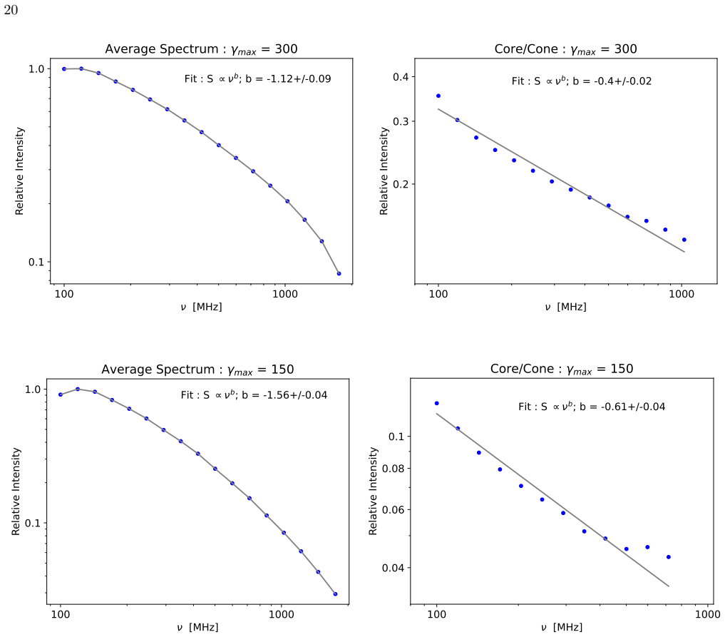
- [3.4, Fig. 10 and Section 3, item 1] The claimed spectral-index agreement is selected rather than predicted. With the default secondary plasma Lorentz-factor range γ_s = 50–300, the model fit gives b = -1.12 ± 0.09; only after reducing the range to γ_s = 50–150 does the fit give b = -1.56 ± 0.04, near the observed median of b ≈ -1.6. No independent physical constraint is given for this reduced upper limit, and the paper explicitly labels the uniform distribution with γ_s between 50 and 300 as the default. As a result, the statement in the Discussion that 'the average spectra from CCR due to charged solitons also show the spectral index to be similar to the median value of the pulsar population' is not supported by the default model. Please treat γ_h as an uncertain parameter, report the spectral index across the full plausible range, and identify an observable that could pin it down.
- [2.2 and 3.1] The reproduction of profile types (M, cQ, T, D, S) is substantially built into the model geometry. In Section 2.2, the sparks are placed in a central core plus one or two concentric rings with angular locations θ' = θ_PC/3, 2θ_PC/5, and 4θ_PC/5, which is exactly the core-cone beam taxonomy used in Section 3.1 to label the resulting profiles. The simulated profiles are then classified with the same core-cone scheme, so the agreement in profile morphology is not an independent confirmation of the soliton CCR mechanism. The RFM, PPA, and spectral results are genuinely emergent, but the profile-shape claim should be reframed or supported by a quantitative comparison that does not presuppose the taxonomy, for example component widths, relative component spacings, or a specific observed pulsar's profile.
- [3, parameter list and Section 4] The model contains several hand-set parameters whose impact on the central conclusions is not quantified in the paper: the group-velocity factor y = 2.3, the soliton length limits Δ_l = 0.4 m and Δ_h = 0.6 m, the coherence parameter a_s = 0.3, and the threshold I_g > 0.001 I_max used to define the emission-height window. Some of these are physically motivated, but the RFM height ranges in Fig. 6 and the width-frequency coefficients in Table 1 depend on the emission-height cutoff and the soliton-length scale. A sensitivity test varying these parameters within their stated ranges (especially y and the threshold) would establish that the qualitative outcomes—RFM, RVM-like PPA, inverted spectra—are robust rather than consequences of the chosen numerical window.
minor comments (5)
- [Table 1] The last row contains a typographical error: for the D-type W_sep fit, the entry reads '-0.29 + ±0.11'; the plus sign before '±' should be removed.
- [2.1 and 2.2] The symbol ρ_s is used for the central charge density inside a soliton in Section 2.1 and for the secondary plasma density distribution in Section 2.2. These are different quantities and the notation should be distinguished to avoid confusion.
- [3.2, Eq. (12) and (13)] The beam opening angle θ_bm^i uses sin^-1 √(r_i/R_LC), and the azimuthal angle formula in Eq. (13) is quoted from Rankin (1993). Please check the limiting behavior at θ_j = 0, where the expression should reduce smoothly; currently it is not obvious that the formula is regular, and a comment or a small limiting form would improve clarity.
- [4, first paragraph] Minor typo: 'open filed line region' should read 'open field line region'.
- [3.1, Figs. 4 and 5] The captions and text refer to the 'right panel' of each figure for the LOS coverage, but in the two-column layout it is the right-hand column; labeling the panels explicitly (a) and (b) in the captions would help the reader.
Assumptions & free parameters
free parameters (5)
- soliton group velocity factor y =
y = 2.3
- secondary plasma Lorentz factor range =
gamma_l = 50, gamma_h = 300, variant gamma_h = 150, step 10
- soliton length limits Delta_l and Delta_h =
0.4 m and 0.6 m at r = 500 km, step 0.1 m
- soliton coherence parameter a_s =
0.3
- emission height cutoff threshold =
I_g > 0.001 I_max
assumptions (6)
- domain assumption Charge-separated solitons form and remain stable in the pulsar plasma, with the charge distribution modeled as three charges per soliton.
- domain assumption Emitted waves propagate as in vacuum; plasma mode splitting, absorption and refraction are ignored.
- domain assumption The emission region is dominated by a purely dipolar field, with spark geometry at the surface following the observed core-cone pattern.
- standard math Standard Airy/Bessel integral representation of ultrarelativistic curvature radiation is valid after dropping the x-squared term in the phase.
- standard math Rotating vector model and aberration-retardation formulas give the PPA and emission-height relation.
- domain assumption Solitons are uniformly distributed along each line of sight and occupy grids with angular spacing 1/(2 y gamma_s).
Cite this review
Pith. "Pith review of Pulsar Coherent Radio Emission from Solitons : Average Emission Properties." pith.science (2026). https://pith.science/paper/M2ND3Q3H
@misc{pith2026250412163,
  author       = {Pith},
  title        = {Pith review of: Pulsar Coherent Radio Emission from Solitons : Average Emission Properties},
  year         = {2026},
  howpublished = {\url{https://pith.science/paper/M2ND3Q3H}},
  note         = {Machine review of arXiv:2504.12163}
}
read the original abstract
Observations have established that coherent radio emission from pulsars arise at few hundred kilometers above stellar surface. Recent polarization studies have further demonstrated that plasma instabilities are necessary for charge bunching that gives rise to coherent emission. The formation of charged solitons in the electron-positron plasma is the only known bunching mechanism that can be realised at these heights. More than five decades of observations have revealed a number of emission features that should emerge from any valid radio emission mechanism. We have carried out numerical calculations to find the features of average emission from curvature radiation due to charged solitons. The characteristic curvature radiation spectrum has been updated from the well known one-dimensional dependence into a general two-dimensional form, and contribution from each soliton along observer's line of sight (LOS) has been added to reproduce the pulsar emission. The outflowing plasma is formed by sparking discharges above the stellar surface that are located within concentric rings resembling the core-cone emission beam, and uniform distribution of solitons along any LOS has been assumed. The observed effects of radius to frequency mapping, where the lower frequency emission originates from higher altitudes, is seen in this setup. The power law spectrum and relative steepening of the core spectra with respect to the cones also emerges. The estimated polarization position angle reflects the geometrical configuration of pulsars as expected. These studies demonstrate the efficacy of coherent curvature radiation from charged solitons to reproduce the average observational features of pulsars.
Figures


Figures from the paper (9 more)




Reference graph
Works this paper leans on
-
[1]
Arons , J., & Barnard , J. J. 1986, , 302, 120, 10.1086/163978
doi:10.1086/163978 1986
-
[2]
2019, , 489, 4589, 10.1093/mnras/stz2299
Arumugasamy , P., & Mitra , D. 2019, , 489, 4589, 10.1093/mnras/stz2299
-
[3]
Asseo , E., & Melikidze , G. I. 1998, , 301, 59, 10.1046/j.1365-8711.1998.01990.x
arXiv 1998
-
[4]
Backer , D. C., & Rankin , J. M. 1980, , 42, 143, 10.1086/190647
doi:10.1086/190647 1980
-
[5]
Basu , R., Melikidze , G. I., & Mitra , D. 2022 a , , 936, 35, 10.3847/1538-4357/ac8479
-
[6]
Basu , R., Mitra , D., & Melikidze , G. I. 2020, , 496, 465, 10.1093/mnras/staa1574
-
[7]
2021, , 917, 48, 10.3847/1538-4357/ac0828
---. 2021, , 917, 48, 10.3847/1538-4357/ac0828
-
[8]
2022 b , , 927, 208, 10.3847/1538-4357/ac5039
---. 2022 b , , 927, 208, 10.3847/1538-4357/ac5039
Show all 66 references
- [9]
-
[10]
I., et al
Basu , R., Mitra , D., Melikidze , G. I., et al. 2016, , 833, 29, 10.3847/1538-4357/833/1/29
2016 doi
-
[11]
I., & Skrzypczak , A
Basu , R., Mitra , D., Melikidze , G. I., & Skrzypczak , A. 2019, , 482, 3757, 10.1093/mnras/sty2846
2019 doi
-
[12]
M., & Wasserman , I
Blaskiewicz , M., Cordes , J. M., & Wasserman , I. 1991, , 370, 643, 10.1086/169850
1991 doi
- [13]
-
[14]
2024, , 974, L32, 10.3847/2041-8213/ad7e24
Chernoglazov , A., Philippov , A., & Timokhin , A. 2024, , 974, L32, 10.3847/2041-8213/ad7e24
2024 doi
-
[15]
Cordes , J. M. 1978, , 222, 1006, 10.1086/156218
1978 doi
-
[16]
2008, , 391, 859, 10.1111/j.1365-2966.2008.13923.x
Dyks , J. 2008, , 391, 859, 10.1111/j.1365-2966.2008.13923.x
2008
-
[17]
Dyks , J., Rudak , B., & Harding , A. K. 2004, , 607, 939, 10.1086/383587
2004 doi
-
[18]
I., & Szkudlarek , M
Geppert , U., Basu , R., Mitra , D., Melikidze , G. I., & Szkudlarek , M. 2021, , 504, 5741, 10.1093/mnras/stab1134
2021 doi
-
[19]
1984, , 132, 312
Gil , J., Gronkowski , P., & Rudnicki , W. 1984, , 132, 312
1984
-
[20]
Gil , J., Lyubarsky , Y., & Melikidze , G. I. 2004, , 600, 872, 10.1086/379972
2004 doi
-
[21]
I., & Geppert , U
Gil , J., Melikidze , G. I., & Geppert , U. 2003, , 407, 315, 10.1051/0004-6361:20030854
2003 doi
-
[22]
A., Kijak , J., & Seiradakis , J
Gil , J. A., Kijak , J., & Seiradakis , J. H. 1993, , 272, 268
1993
- [23]
-
[24]
A., Melikidze , G
Gil , J. A., Melikidze , G. I., & Mitra , D. 2002, , 388, 235, 10.1051/0004-6361:20020473
2002 doi
- [25]
-
[26]
Goldreich , P., & Julian , W. H. 1969, , 157, 869, 10.1086/150119
1969 doi
-
[27]
A., Kuzmin , A
Izvekova , V. A., Kuzmin , A. D., Malofeev , V. M., & Shitov , I. P. 1981, , 78, 45, 10.1007/BF00654022
1981 doi
-
[28]
Jackson , J. D. 1998, Classical Electrodynamics, 3rd Edition
1998
-
[29]
F., et al
Jankowski , F., van Straten , W., Keane , E. F., et al. 2018, , 473, 4436, 10.1093/mnras/stx2476
2018 doi
-
[30]
2021, , 923, 211, 10.3847/1538-4357/ac3082
Kijak , J., Basu , R., Lewandowski , W., & Ro \.z ko , K. 2021, , 923, 211, 10.3847/1538-4357/ac3082
2021 doi
-
[31]
1997, , 288, 631, 10.1093/mnras/288.3.631
Kijak , J., & Gil , J. 1997, , 288, 631, 10.1093/mnras/288.3.631
1997 doi
-
[32]
2011, , 531, A16, 10.1051/0004-6361/201014274
Kijak , J., Lewandowski , W., Maron , O., Gupta , Y., & Jessner , A. 2011, , 531, A16, 10.1051/0004-6361/201014274
2011 doi
-
[33]
2018, , 480, 4526, 10.1093/mnras/sty2152
Lakoba , T., Mitra , D., & Melikidze , G. 2018, , 480, 4526, 10.1093/mnras/sty2152
2018 doi
-
[34]
2012, , 424, 1762, 10.1111/j.1365-2966.2012.21246.x
Maciesiak , K., Gil , J., & Melikidze , G. 2012, , 424, 1762, 10.1111/j.1365-2966.2012.21246.x
2012
-
[35]
2000, , 147, 195, 10.1051/aas:2000298
Maron , O., Kijak , J., Kramer , M., & Wielebinski , R. 2000, , 147, 195, 10.1051/aas:2000298
2000 doi
-
[36]
I., Gil , J
Melikidze , G. I., Gil , J. A., & Pataraya , A. D. 2000, , 544, 1081, 10.1086/317220
2000 doi
-
[37]
I., & Pataraia , A
Melikidze , G. I., & Pataraia , A. D. 1980, Astrofizika, 16, 161
1980
-
[38]
2017, Journal of Astrophysics and Astronomy, 38, 52, 10.1007/s12036-017-9457-6
Mitra , D. 2017, Journal of Astrophysics and Astronomy, 38, 52, 10.1007/s12036-017-9457-6
2017 doi
-
[39]
2016, , 833, 28, 10.3847/1538-4357/833/1/28
Mitra , D., Basu , R., Maciesiak , K., et al. 2016, , 833, 28, 10.3847/1538-4357/833/1/28
2016 doi
-
[40]
Mitra , D., Basu , R., & Melikidze , G. I. 2024 a , , 974, 254, 10.3847/1538-4357/ad71ca
2024 doi
-
[41]
I., & Arjunwadkar , M
Mitra , D., Basu , R., Melikidze , G. I., & Arjunwadkar , M. 2020, , 492, 2468, 10.1093/mnras/stz3620
2020 doi
-
[42]
Mitra , D., Basu , R., & Melikizde , G. I. 2024 b , Universe, 10, 248, 10.3390/universe10060248
2024 doi
-
[43]
Mitra , D., & Deshpande , A. A. 1999, , 346, 906. astro-ph/9904336
1999 arXiv
-
[44]
Mitra , D., & Li , X. H. 2004, , 421, 215, 10.1051/0004-6361:20034094
2004 doi
-
[45]
I., & Basu , R
Mitra , D., Melikidze , G. I., & Basu , R. 2023 a , , 952, 151, 10.3847/1538-4357/acdc28
2023 doi
-
[46]
2023 b , , 521, L34, 10.1093/mnrasl/slad022
---. 2023 b , , 521, L34, 10.1093/mnrasl/slad022
2023 doi
-
[47]
Mitra , D., & Rankin , J. M. 2002, , 577, 322, 10.1086/342136
2002 doi
-
[48]
Olszanski , T. E. E., Mitra , D., & Rankin , J. M. 2019, , 489, 1543, 10.1093/mnras/stz2172
2019 doi
-
[49]
2016, Journal of Plasma Physics, 82, 635820502, 10.1017/S0022377816000763
P \'e tri , J. 2016, Journal of Plasma Physics, 82, 635820502, 10.1017/S0022377816000763
2016 doi
-
[50]
2020, , 491, 80, 10.1093/mnras/stz2974
P \'e tri , J., & Mitra , D. 2020, , 491, 80, 10.1093/mnras/stz2974
2020 doi
-
[51]
Radhakrishnan , V., & Cooke , D. J. 1969, , 3, 225
1969
-
[52]
M., Mitra , D., & Melikidze , G
Rahaman , S. M., Mitra , D., & Melikidze , G. I. 2020, , 497, 3953, 10.1093/mnras/staa2280
2020 doi
-
[53]
M., Mitra , D., Melikidze , G
Rahaman , S. M., Mitra , D., Melikidze , G. I., & Lakoba , T. 2022, , 516, 3715, 10.1093/mnras/stac2264
2022 doi
-
[54]
Rankin , J. M. 1983, , 274, 333, 10.1086/161450
1983 doi
- [55]
- [56]
-
[57]
A., & Sutherland , P
Ruderman , M. A., & Sutherland , P. G. 1975, , 196, 51, 10.1086/153393
1975 doi
-
[58]
1997, , 321, 519
Sieber , W. 1997, , 321, 519
1997
-
[59]
Sturrock , P. A. 1971, , 164, 529, 10.1086/150865
1971 doi
-
[60]
2017, , 835, 178, 10.3847/1538-4357/835/2/178
Szary , A., Gil , J., Zhang , B., et al. 2017, , 835, 178, 10.3847/1538-4357/835/2/178
2017 doi
-
[61]
2020, , 493, 3770, 10.1093/mnras/staa492
Sznajder , M., & Geppert , U. 2020, , 493, 3770, 10.1093/mnras/staa492
2020 doi
-
[62]
Thorsett , S. E. 1991, , 377, 263, 10.1086/170355
1991 doi
-
[63]
N., & Harding , A
Timokhin , A. N., & Harding , A. K. 2019, , 871, 12, 10.3847/1538-4357/aaf050
2019 doi
-
[64]
Usov , V. V. 1987, , 320, 333, 10.1086/165546
1987 doi
-
[65]
T., & Stappers , B
Weltevrede , P., Edwards , R. T., & Stappers , B. W. 2006, , 445, 243, 10.1051/0004-6361:20053088
2006 doi
-
[66]
2018, , 868, 31, 10.3847/1538-4357/aae685
Yang , Y.-P., & Zhang , B. 2018, , 868, 31, 10.3847/1538-4357/aae685
2018 doi
Reviewed August 16, 2026 · model on record in the stance chip above.
Discussion (0). Continue with ORCID to comment.