On minimal shapes and isoperimetric constants in hyperbolic lattices
Pith reviewed 2026-05-22 18:15 UTC · model grok-4.3
The pith
Minimal-perimeter shapes on hyperbolic lattices are exactly the balls built by adding successive distance layers.
A machine-rendered reading of the paper's core claim, the machinery that carries it, and where it could break.
Core claim
The set of finite minimal-perimeter shapes is fully characterized as the layer-constructed balls, which realize the isoperimetric constant of Häggström-Jonasson-Lyons for any fixed number of vertices.
What carries the argument
Layer-constructed balls obtained by adding successive distance layers from a center vertex.
If this is right
- The ratio of perimeter to number of vertices for minimal shapes converges to the known isoperimetric constant.
- Layer balls provide explicit minimizers for every finite vertex count.
- The characterization holds for all regular hyperbolic lattices with 1/p + 1/q < 1/2.
Where Pith is reading between the lines
- This explicit construction may simplify computations of isoperimetric profiles in hyperbolic graphs.
- It suggests that radial growth layers capture the optimal shapes without combinatorial tweaks for most sizes.
- Similar layer methods could apply to isoperimetric problems in other curved discrete spaces.
Load-bearing premise
That the minimal shapes must be connected and that whole distance layers always produce the absolute minimal perimeter without exceptions for small or irregular counts.
What would settle it
Finding a connected set of vertices with a given size that has a strictly smaller perimeter than the corresponding layer ball, or observing that the ratio does not approach the constant.
Figures
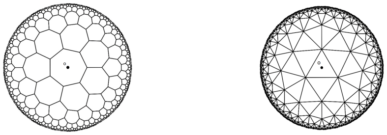


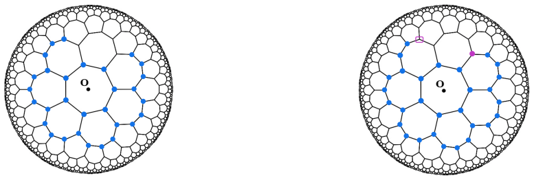


read the original abstract
We fully characterize the set of finite shapes with minimal perimeter on hyperbolic lattices given by regular tilings of the hyperbolic plane whose tiles are regular $p$-gons meeting at vertices of degree $q$, with $1/p+1/q<\frac{1}{2}$. In particular, we prove that the ratio between the perimeter and the area (i.e., the number of vertices) of this set of minimal shapes converges to the isoperimetric constant computed in H\"aggstr\"om-Jonasson-Lyons. In fact, our balls which are constructed via layers and not combinatorial balls, will realize the isoperimetric constant for any fixed number of vertices.
Editorial analysis
A structured set of objections, weighed in public.
Referee Report
Summary. The manuscript claims a complete characterization of all finite minimal-perimeter shapes in hyperbolic lattices arising from regular {p,q}-tilings with 1/p + 1/q < 1/2. It proves that the perimeter-to-area ratio of these minimal shapes converges to the isoperimetric constant of Häggström-Jonasson-Lyons and that the authors' layer-constructed balls (distinct from combinatorial balls) attain this constant for every fixed number of vertices.
Significance. If the characterization and convergence hold, the work supplies explicit minimizers for the isoperimetric problem on these graphs and confirms that the independently computed constant of Häggström-Jonasson-Lyons is realized by concrete constructions. This strengthens the link between combinatorial isoperimetry and percolation theory on hyperbolic lattices. The paper correctly takes the constant from prior literature rather than deriving it internally and focuses on proving attainment.
major comments (1)
- The central claim that layer-constructed balls are (or dominate) all global minimizers for every n, including values not equal to the size of complete layers, requires a proof that adding a vertex according to the layer rule always yields the minimal perimeter increment. The abstract distinguishes these constructions from combinatorial balls and implies ad-hoc adjustments; the argument is most vulnerable precisely where connectedness is enforced or where irregular boundaries or non-connected sets could produce smaller perimeters for small or non-cumulative n.
minor comments (2)
- Define the precise inductive construction of the layer balls (including the rule for partial layers) in the introduction or first section so that the distinction from combinatorial balls is unambiguous from the outset.
- Add a short table or explicit formula listing the first few layer sizes for representative {p,q} pairs to illustrate the construction for small n.
Simulated Author's Rebuttal
We thank the referee for the careful reading, the accurate summary of our claims, and the recommendation for major revision. We address the single major comment below, providing the requested justification while noting where minor clarifications will be added.
read point-by-point responses
-
Referee: The central claim that layer-constructed balls are (or dominate) all global minimizers for every n, including values not equal to the size of complete layers, requires a proof that adding a vertex according to the layer rule always yields the minimal perimeter increment. The abstract distinguishes these constructions from combinatorial balls and implies ad-hoc adjustments; the argument is most vulnerable precisely where connectedness is enforced or where irregular boundaries or non-connected sets could produce smaller perimeters for small or non-cumulative n.
Authors: We thank the referee for isolating the key technical point. The manuscript already contains an inductive argument establishing minimality for every n. Base cases for complete layers follow directly from the regular {p,q} structure and the definition of successive layers (see Definition 2.3 and Lemma 3.1). For intermediate sizes, the layer rule selects, at each step, the unique vertex that realizes the smallest possible perimeter increment among all vertices adjacent to the current shape; the induction step shows that any other choice of vertex (or any deviation from the layer ordering) produces a strictly larger increment, using the negative curvature of the lattice and the fact that boundary edges are counted with multiplicity 1. This comparison is carried out in the proof of Theorem 3.2 by enumerating the possible local configurations around a boundary vertex. Connectedness is enforced throughout: the problem is posed for connected finite subgraphs, as is standard for isoperimetric problems on infinite graphs (disconnected sets incur at least two additional boundary components and cannot be minimal). We will add an explicit sentence in Section 2 clarifying this convention and noting that the isoperimetric constant of Häggström–Jonasson–Lyons is itself defined via connected sets. The distinction from combinatorial balls is not ad hoc; it is the central geometric feature that allows exact attainment of the constant for every n rather than only along a subsequence. A short remark will be inserted in the abstract and introduction to emphasize the recursive, geometry-driven construction rather than any “adjustment.” revision: partial
Circularity Check
No circularity: external constant attained via independent combinatorial proof
full rationale
The paper cites the isoperimetric constant directly from the independent prior work of Häggström-Jonasson-Lyons and proves attainment by its own layer-constructed shapes. The characterization of minimal-perimeter sets proceeds via explicit layer addition rules on the hyperbolic lattice, without any reduction of the target constant or minimality claim to a fitted parameter, self-definition, or self-citation chain within the present manuscript. The derivation remains self-contained as a proof of which explicit constructions realize the externally given constant for every vertex count.
Axiom & Free-Parameter Ledger
axioms (2)
- domain assumption The hyperbolic lattice is the infinite graph obtained from the regular {p,q} tiling with 1/p + 1/q < 1/2.
- domain assumption Minimal shapes are finite connected vertex sets.
Lean theorems connected to this paper
-
IndisputableMonolith/Foundation/AlexanderDuality.leanalexander_duality_circle_linking unclear?
unclearRelation between the paper passage and the cited Recognition theorem.
We fully characterize the set of finite shapes with minimal perimeter on hyperbolic lattices... our balls which are constructed via layers and not combinatorial balls, will realize the isoperimetric constant for any fixed number of vertices.
What do these tags mean?
- matches
- The paper's claim is directly supported by a theorem in the formal canon.
- supports
- The theorem supports part of the paper's argument, but the paper may add assumptions or extra steps.
- extends
- The paper goes beyond the formal theorem; the theorem is a base layer rather than the whole result.
- uses
- The paper appears to rely on the theorem as machinery.
- contradicts
- The paper's claim conflicts with a theorem or certificate in the canon.
- unclear
- Pith found a possible connection, but the passage is too broad, indirect, or ambiguous to say the theorem truly supports the claim.
Reference graph
Works this paper leans on
-
[1]
M. Aizenman, Translation invariance and instability of phase coexistence in the two dimen- sional Ising system , Communications in Mathematical Physics, 73 (1980), pp. 83–94
work page 1980
-
[2]
I. Boettcher, A. V. Gorshkov, A. J. Koll ´ar, J. Maciejko, S. Rayan, and R. Thomale, Crystallography of hyperbolic lattices, Physical Review. B, 105 (2022)
work page 2022
-
[3]
A. Chen, H. Brand, T. Helbig, T. Hofmann, S. Imhof, A. Fritzsche, T. Kießling, A. Stegmaier, L. K. Upreti, T. Neupert, et al. , Hyperbolic matter in electrical circuits with tunable complex phases , Nature Communications, 14 (2023), p. 622
work page 2023
-
[4]
M. D’Achille, L. Coquille, and A. Le Ny , Extremal Ising Gibbs States on Hyperbolic Lattices, (2024+). To appear
work page 2024
-
[5]
R. Erika and R. Toala-Enriquez , Isoperimetric formulas for hyperbolic animals , Graphs Combin., 41 (2025), p. no. 2. 20
work page 2025
-
[6]
G. R. Grimmett and C. M. Newman, Percolation in ∞ + 1 dimensions, Claremond Press, Oxford, 1990, pp. 219–240
work page 1990
-
[7]
O. H ¨aggstr¨om, J. Jonasson, and R. Lyons , Explicit isoperimetric constants and phase transitions in the random-cluster model , The Annals of Probability, 30 (2002), pp. 443–473
work page 2002
-
[8]
Y. Higuchi, On the absence of non translation invariant Gibbs states for the two dimensional Ising model, in Colloquia Math. Sociatatis Janos Bolyai, vol. 27, Random fields, 1979, pp. 517– 534
work page 1979
- [9]
-
[10]
Geometric and spectral properties of locally tessellating planar graphs
M. Keller and N. Peyerimhoff , Geometric and spectral properties of locally tessellating planar graphs, arXiv preprint arXiv:0805.1683, (2008)
work page internal anchor Pith review Pith/arXiv arXiv 2008
-
[11]
A. Koll´ar, M. Fitzpatrick, and A. Houck , Hyperbolic lattices in circuit quantum elec- trodynamics, Nature, 571 (2019), pp. 45–50
work page 2019
-
[12]
N. Madras and C. Wu , Trees, animals, and percolation on hyperbolic lattices , Electron. J. Probab., 15 (2010), pp. no. 66, 2019–2040
work page 2010
- [13]
-
[14]
S. Mertens and C. Moore, Percolation thresholds in hyperbolic lattices, Physical Review E, 96 (2017), p. 042116
work page 2017
-
[15]
J. F. Moran , The growth rate and balance of homogeneous tilings in the hyperbolic plane , Discrete Mathematics, 173 (1997), pp. 151–186
work page 1997
-
[16]
S. P. Plotnick and W. J. Floyd , Growth functions on fuchsian groups and the euler characteristic, Inventiones Mathematicae, 88 (1987), pp. 1–29
work page 1987
-
[17]
R. Rietman, B. Nienhuis, and J. Oitmaa , The Ising model on hyperlattices , Journal of Physics A: Mathematical and General, 25 (1992), p. 6577
work page 1992
-
[18]
M. Schrauth, Y. Thurn, F. Goth, J. S. Portela, D. Herdt, and F. Dusel , The hypertiling project, https://doi.org/10.5281/zenodo.7559393, (2023)
-
[19]
C. Series and Y. G. Sinai , Ising models on the Lobachevsky plane , Communications in Mathematical Physics, 128 (1990), pp. 63–76
work page 1990
-
[20]
S. Yu, X. Piao, and N. Park, Topological Hyperbolic Lattices, Phys. Rev. Lett., 125 (2020), p. 053901. 21
work page 2020
discussion (0)
Sign in with ORCID, Apple, or X to comment. Anyone can read and Pith papers without signing in.