REVIEW 3 major objections 5 minor 55 references
Conditional flow matching for generative modeling of near-wall turbulence with quantified uncertainty
T0 review · 3 major / 5 minor · reviewed 2026-08-16 · deepseek-v4-flash
Pith's one-line read A flow-matching generative model, trained once without labels, reconstructs instantaneous near-wall velocity fluctuations at three wall-normal heights from sparse wall shear stress and pressure, with per-sample uncertainty that grows as…
desk verdict A solid first application of training-free flow matching to near-wall turbulence reconstruction, undermined by an unfair baseline comparison that should be fixed before acceptance. read the letter →
The pith
A machine-rendered reading of the paper's core claim, the machinery that carries it, and where it could break.
The reading
What carries the argument
The load-bearing mechanism is training-free predictor-corrector guidance for the flow-matching ODE. The learned transport velocity $\nu_\theta(\tau, x_\tau)$ in $\mathrm{d}x_\tau/\mathrm{d}\tau = \nu_\theta(\tau, x_\tau)$ carries samples from Gaussian noise to the turbulence distribution, and at inference a correction term is added that points along the normalized gradient of the measurement mismatch, $\nu' = -b\,\|\nu_\theta\|\, \nabla_{x_\tau} D(\hat{y}, y)/\|\nabla_{x_\tau} D(\hat{y}, y)\|$. The mismatch is evaluated through a one-step linear extrapolation of the terminal state, $\hat{x}_{1|\tau} = x_\tau + (1-\tau)\nu_\theta(\tau, x_\tau)$, fed into a patch-trained, fully convolutional U-Net forward operator that predicts wall quantities with quantified epistemic uncertainty from SWAG weight samples. The scalar guidance strength $b$ balances the prior flow against the data correction, and the SWAG covariance makes the gradient itself uncertain, so weak or sparse wall coupling naturally produces wider predictive ensembles.
What would settle it
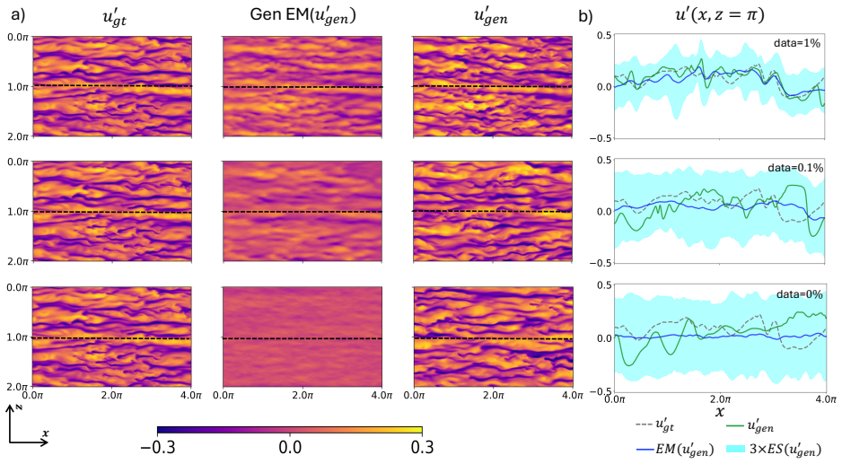
Integrate the flow ODE without guidance to obtain the exact terminal endpoint for a set of intermediate states and compare it with the one-step extrapolation of Eq. (9): if the two diverge substantially at early times $\tau$, the correction gradients are computed from a biased target and the measurement-consistency results should degrade. A second, purely behavioral check: across the coverage levels 100%, 10%, 1%, 0.1%, and 0%, the ensemble standard deviation must grow monotonically with sparsity and the normalized wall-measurement error $\Delta_y$ must fall below the unconditional baseline, so a non-monotonic uncertainty curve, or conditional samples no more measurement-consistent than unconditional ones, would contradict the central claims.
Extended reading notes
Core claim
The central claim is that zero-shot conditional generation of near-wall turbulence is achievable by combining continuous-time flow matching with a probabilistic forward operator trained using stochastic weight averaging Gaussian (SWAG), a Bayesian technique that approximates a distribution over network weights rather than a single estimate. The generative model learns the unconditional distribution of instantaneous velocity fluctuations at $y^+ = 5$, $20$, and $40$ from DNS data, while the forward operator learns the noisy, uncertain mapping from such velocity fields to wall shear stress and pressure. At inference, the flow ODE is integrated with the added correction $\nu'(\tau, x_\tau, y) = -b\,\|\nu_\theta(\tau, x_\tau)\|\, \nabla_{x_\tau} D(\hat{y}, y) / \|\nabla_{x_\tau} D(\hat{y}, y)\|$, where the mismatch $D(\hat{y}, y)$ is computed by extrapolating the current state one step toward its terminal endpoint, passing it through the differentiable forward operator, and differentiating the resulting measurement error. The authors show that this procedure yields ensembles whose mean tracks the DNS ground truth across all three wall-normal positions, whose individual members keep small-scale intermittency even where the mean is smooth, whose two-dimensional energy spectra agree with DNS statistics, and whose spread widens as wall data thins from 100% to 10% to 1% to 0%, with the widest band at $y^+=20$ coinciding with the peak turbulence intensity of the buffer layer.
Load-bearing premise
The load-bearing approximation is that the one-step linear extrapolation of Eq. (9) faithfully estimates the terminal state of the flow for the purpose of computing measurement-mismatch gradients, and that a hand-tuned scalar guidance strength $b$ keeps this correction balanced against the learned transport velocity, so that if either assumption gives way, the zero-shot conditioning would no longer steer generated samples toward the observed wall data.
Editorial extensions
If this is right
- Reconstruction of off-wall velocity from wall-mounted sensors becomes feasible for closed-loop flow control and real-time monitoring, because the same pretrained model accepts any differentiable observation operator without retraining.
- Predictive uncertainty is reported per sample and tracks physical observability: the ensemble widens with wall distance, peaks at the buffer-layer height $y^+=20$ where turbulence intensity is largest, and grows monotonically as wall coverage falls.
- Under 10% wall data the generated energy spectra remain close to DNS, whereas the CNN and linear stochastic estimation baselines produce over-smoothed or spectrally depleted fields, so usable reconstruction extends into the weakly observable regime where deterministic estimators fail.
- The SWAG forward operator also functions as a candidate data-driven wall model: in an a priori test it reproduces DNS wall shear stress statistics more closely than a Spalding algebraic wall model, pointing toward wall-modeled large-eddy simulation.
Reading between the lines
- The correction term is a variational approximation to the gradient of the log-posterior, and if that reading is correct the hand-tuned strength $b$ could be replaced by a calibrated schedule fitted on a validation set, turning the ensemble spread into a principled posterior standard deviation.
- Because the framework is agnostic to the observation operator, the same pretrained flow-matching prior should assimilate other measurement modalities — Lagrangian particle tracks, planar PIV slices, or sparse in-domain velocity probes — by swapping only the differentiable forward map; this is a testable extension the paper gestures toward but does not run.
- The non-monotonic uncertainty peak at $y^+=20$ suggests the ensemble spread encodes intrinsic buffer-layer dynamics rather than mere observability, and if it persists at higher Reynolds numbers the spread could serve as a diagnostic of near-wall activity instead of a simple error bar.
Signed reviews
Editorial analysis
A structured set of objections, weighed in public.
Referee Report
Summary. The paper proposes a generative framework for reconstructing instantaneous velocity fluctuation fields in turbulent channel flow (Re_tau=180) at wall-normal positions y+ = 5, 20, and 40 from wall measurements. The method combines a flow-matching generative model for velocity fields with a stochastic weight averaging Gaussian (SWAG) probabilistic forward operator mapping velocity to wall quantities. Conditioning is performed at test time by adding a gradient-based correction term to the flow-matching ODE, allowing zero-shot adaptation to sparse, partial, and low-resolution wall data without retraining. The authors evaluate the framework on held-out DNS data using qualitative visualizations, correlation coefficients, energy spectra, and uncertainty bands, and compare against CNN and LSE baselines. They report superior fidelity and robustness under 10% wall data and argue that the framework preserves turbulence statistics while providing quantified epistemic uncertainty.
Significance. If the central claims are supported, this is a timely and useful contribution. The paper is, to my knowledge, the first to apply flow matching to 3D inhomogeneous and anisotropic near-wall turbulence reconstruction with explicit uncertainty quantification, and the test-time conditioning strategy addresses a practical need for sensor-configuration flexibility. The strongest aspects are the spectral validation of generated fields against DNS on a held-out set of 500 independent samples, the systematic study of uncertainty growth with wall distance and sensor sparsity, and the demonstration of conditioning under several realistic measurement degradations. The work is empirical but internally consistent: the forward operator is trained on distinct velocity-wall pairs and the test set is held out, so the conditioning is not circular in a data sense. However, the uncertainty estimates are never calibrated against ground-truth coverage, and the baseline comparison contains a potential train/test distribution mismatch that directly affects the paper's headline claim of superior generalization under sparsity.
major comments (3)
- [§4.1, Figures 10-11] The claim of superior resilience under 10% wall data is not established because the CNN and LSE baselines appear to be trained on full-resolution wall inputs and then evaluated on sparse masks. The CNN baseline is described in Appendix B as learning a mapping from wall quantities to velocity (following Guastoni et al. [22]), and the LSE kernel h in Eq. (22) is fit over the training dataset; neither is described as retrained with random masks or given the mask as an additional input. The proposed method, by contrast, is explicitly designed for arbitrary masks via the test-time guidance in Eqs. (8)-(11). If the baselines receive only 10% of the inputs they were trained on, their near-zero correlations and collapsing spectra in Figure 11 reflect input distribution shift rather than an intrinsic limitation of deterministic estimators. The manuscript must state whether the baselines were retrained with the same random masks (or mask-aware training) for each sparsity level; if not, the comparison should be rerun under matched training conditions before the superiority claim is made.
- [§3.4, Figures 5-7] The uncertainty quantification is never calibrated against ground-truth coverage. The ensemble spread (ES) and scalar STD in Eq. (21) are reported and shown to grow with wall distance and sparsity, but the manuscript does not report the fraction of ground-truth points within the stated confidence intervals (e.g., 3×ES in Figure 5b) or any reliability/coverage diagnostic. Without such calibration, the interpretability of the uncertainty bands is unclear, and the claim of 'quantified uncertainty' is incomplete. Please add a coverage analysis over the 500 test cases for representative configurations, or explicitly state that the ensemble spread is a relative measure not intended as calibrated posterior intervals.
- [§2.4, Eqs. (9) and (11)] The zero-shot conditioning mechanism relies on two heuristics that are not validated: the one-step linear extrapolation x1_hat = x_tau + (1-tau) nu_theta(tau, x_tau) in Eq. (9), and the normalized-gradient correction with norm matching in Eq. (11). The paper states that the latter 'can be viewed as a variational approximation' to the log-posterior gradient, but no derivation or error bound is provided, and the guidance strength b is hand-tuned. The central claim of training-free conditional generation depends on these approximations. Please provide a sensitivity analysis of b (and measurement noise sigma_e) on reconstruction fidelity, and compare the one-step extrapolation against a multi-step or exact endpoint estimate on a subset of test cases. Without this, the reader cannot assess whether the reported results are robust or specific to the chosen hyperparameters.
minor comments (5)
- [§3.4, Figure 7] The scalar metrics r and STD in Figure 7 are reported as single points per configuration without error bars or variability across ensemble seeds; given that Nens = 50, bootstrap intervals would strengthen the quantitative claims.
- [§2.3, Eq. (7)] The notation x1 is used both for a target data sample and for the endpoint of the flow; consider clarifying to avoid confusion in Eqs. (7)-(9).
- [§3.5, Figure 8] The caption of Figure 8 refers to '500 different test wall measurements' but the panel shows only one example; make clear that the PDF in panel (d) is computed over the full test set.
- [Appendix A, Table A.2] The flow-matching network has about 105 million parameters and the measurement operator about 7.9 million; reporting training time and hardware would help readers gauge practical applicability.
- [§2.5, Eq. (12)] The SWAG covariance notation in Eq. (13) uses phi^2 and phi_SWA^2, which is nonstandard; define the squaring as element-wise and specify that phi_SWA is the running average over SGD iterates.
Circularity Check
No significant circularity: conditional generation is a genuine zero-shot optimization against held-out wall measurements, and the self-citations are contextual rather than load-bearing.
full rationale
The paper's derivation chain is not circular. The flow-matching generative model is trained unconditionally on velocity fluctuation snapshots only (Section 2.3, Eq. 7), while the SWAG-based forward operator is trained separately on roughly 9,000 velocity-to-wall pairs (Section 2.5), and evaluation is performed on an independent set of 500 held-out samples (Section 3.1). At inference, the guidance correction in Eqs. (8)-(11) uses the learned forward operator to compare predicted wall quantities against the actual wall measurements; the measurements y are external held-out inputs, not values fitted from the generated velocity fields, and the forward operator was fit on a different subset of data. Therefore the 'predicted' velocity fields are not equal to the fitted forward-operator outputs by construction. The energy-spectrum agreement with DNS (Figures 3c, 4c, 10) is a post-hoc statistical validation against the reference distribution, not a constraint used to construct the samples, so it is also not circular. The self-citations (Refs. [42], [44]) describe prior generative turbulence work and are contextual; the load-bearing algorithmic components (flow matching from Lipman et al., SWAG from Maddox et al., and diffusion posterior sampling from Chung et al.) are external, peer-reviewed, or code-reproducible sources. No uniqueness theorem is imported from the authors' prior work, and no ansatz is smuggled in solely by self-citation; the one-step terminal-state approximation in Eq. (9) is explicitly presented as a heuristic approximation. The main caveat is a baseline-comparison fairness question: Sections 4.1 and Appendix B do not state whether the CNN and LSE baselines were retrained or mask-conditioned for the sparse sensor cases in Figures 10-11. That concern is about experimental validity and train/test distribution mismatch, not circularity, and it does not affect the internal derivation chain of the proposed framework.
Assumptions & free parameters
free parameters (4)
- guidance strength b
- measurement noise sigma_e
- sigma_min
- number of sampling steps / solver settings
assumptions (4)
- standard math Flow matching conditional loss gradient equivalence, nabla_theta L = nabla_theta tilde L, and the interpolation path properties from Lipman et al. (2022).
- ad hoc to paper A one-step linear extrapolation x1_hat = x_tau + (1-tau) nu_theta(tau, x_tau) accurately approximates the true endpoint of the flow.
- domain assumption The DNS dataset at Re_tau = 180 is representative of near-wall turbulence physics relevant to real flows.
- ad hoc to paper The normalized gradient update with norm matching to ||nu_theta|| (Eq. 11) acts as a valid variational approximation to the log-posterior gradient.
Cite this review
Pith. "Pith review of Conditional flow matching for generative modeling of near-wall turbulence with quantified uncertainty." pith.science (2026). https://pith.science/paper/J4HOIK6I
@misc{pith2026250414485,
  author       = {Pith},
  title        = {Pith review of: Conditional flow matching for generative modeling of near-wall turbulence with quantified uncertainty},
  year         = {2026},
  howpublished = {\url{https://pith.science/paper/J4HOIK6I}},
  note         = {Machine review of arXiv:2504.14485}
}
read the original abstract
Reconstructing near-wall turbulence from wall-based measurements is a critical yet inherently ill-posed problem in wall-bounded flows, where limited sensing and spatially heterogeneous flow-wall coupling challenge deterministic estimation strategies. To address this, we introduce a novel generative modeling framework based on conditional flow matching for synthesizing instantaneous velocity fluctuation fields from wall observations, with explicit quantification of predictive uncertainty. Our method integrates continuous-time flow matching with a probabilistic forward operator trained using stochastic weight averaging Gaussian (SWAG), enabling zero-shot conditional generation without model retraining. We demonstrate that the proposed approach not only recovers physically realistic, statistically consistent turbulence structures across the near-wall region but also effectively adapts to various sensor configurations, including sparse, incomplete, and low-resolution wall measurements. The model achieves robust uncertainty-aware reconstruction, preserving flow intermittency and structure even under significantly degraded observability. Compared to classical linear stochastic estimation (LSE) and deterministic convolutional neural networks (CNN) methods, our stochastic generative learning framework exhibits superior generalization and resilience under measurement sparsity with quantified uncertainty. This work establishes a robust semi-supervised generative modeling paradigm for data-consistent flow reconstruction and lays the foundation for uncertainty-aware, sensor-driven modeling of wall-bounded turbulence.
Figures


Figures from the paper (12 more)




Reference graph
Works this paper leans on
-
[22]
L. Guastoni, A. G¨ uemes, A. Ianiro, S. Discetti, P. Schlatter, H. Azizpour, R. Vinuesa, Convolutional-network models to predict wall-bounded turbulence from wall quantities, Jour- nal of Fluid Mechanics 928 (2021) A27
work page 2021
-
[1]
Townsend, Equilibrium layers and wall turbulence, Journal of Fluid Mechanics 11 (1) (1961) 97–120
A. Townsend, Equilibrium layers and wall turbulence, Journal of Fluid Mechanics 11 (1) (1961) 97–120
work page 1961
-
[2]
S. B. Pope, Turbulent flows, Measurement Science and Technology 12 (11) (2001) 2020–2021
2001
-
[3]
R. J. Adrian, Hairpin vortex organization in wall turbulence, Physics of fluids 19 (4) (2007)
work page 2007
- [4]
-
[5]
J. Kim, Active control of turbulent boundary layers for drag reduction, in: Industrial and Environmental Applications of Direct and Large-Eddy Simulation: Proceedings of a Workshop Held in Istanbul, Turkey, 5–7 August 1998, Springer, 2007, pp. 142–152
work page 1998
-
[6]
L. L¨ ofdahl, M. Gad-el Hak, Mems-based pressure and shear stress sensors for turbulent flows, Measurement Science and Technology 10 (8) (1999) 665
work page 1999
-
[7]
H. Choi, P. Moin, J. Kim, Active turbulence control for drag reduction in wall-bounded flows, Journal of Fluid Mechanics 262 (1994) 75–110. 36
work page 1994
Show all 55 references
-
[8]
T. A. Zaki, Turbulence from an observer perspective, Annual Review of Fluid Mechanics 57 (2024)
2024
-
[9]
H. Abe, H. Kawamura, H. Choi, Very large-scale structures and their effects on the wall shear- stress fluctuations in a turbulent channel flow up to re τ= 640, J. Fluids Eng. 126 (5) (2004) 835–843
2004
-
[10]
Mathis, N
R. Mathis, N. Hutchins, I. Marusic, Large-scale amplitude modulation of the small-scale struc- tures in turbulent boundary layers, Journal of Fluid Mechanics 628 (2009) 311–337
2009
-
[11]
Lozano-Dur´ an, J
A. Lozano-Dur´ an, J. Jim´ enez, Time-resolved evolution of coherent structures in turbulent channels: characterization of eddies and cascades, Journal of fluid mechanics 759 (2014) 432– 471
2014
-
[12]
Colburn, J
C. Colburn, J. Cessna, T. Bewley, State estimation in wall-bounded flow systems. part 3. the ensemble kalman filter, Journal of Fluid Mechanics 682 (2011) 289–303
2011
-
[13]
M. Wang, T. A. Zaki, Variational data assimilation in wall turbulence: from outer observations to wall stress and pressure, Journal of Fluid Mechanics 1008 (2025) A26
2025
-
[14]
Suzuki, Y
T. Suzuki, Y. Hasegawa, Estimation of turbulent channel flow at based on the wall measure- ment using a simple sequential approach, Journal of Fluid Mechanics 830 (2017) 760–796
2017
-
[15]
F. R. Amaral, A. V. Cavalieri, E. Martini, P. Jordan, A. Towne, Resolvent-based estimation of turbulent channel flow using wall measurements, Journal of Fluid Mechanics 927 (2021) A17
2021
-
[16]
R. J. Adrian, P. Moin, Stochastic estimation of organized turbulent structure: homogeneous shear flow, Journal of Fluid Mechanics 190 (1988) 531–559
1988
-
[17]
Marusic, R
I. Marusic, R. Mathis, N. Hutchins, Predictive model for wall-bounded turbulent flow, Science 329 (5988) (2010) 193–196
2010
-
[18]
W. J. Baars, N. Hutchins, I. Marusic, Spectral stochastic estimation of high-reynolds-number wall-bounded turbulence for a refined inner-outer interaction model, Physical Review Fluids 1 (5) (2016) 054406. 37
2016
-
[19]
M. P. Encinar, J. Jim´ enez, Logarithmic-layer turbulence: a view from the wall, Physical Review Fluids 4 (11) (2019) 114603
2019
-
[20]
Towne, O
A. Towne, O. T. Schmidt, T. Colonius, Spectral proper orthogonal decomposition and its re- lationship to dynamic mode decomposition and resolvent analysis, Journal of Fluid Mechanics 847 (2018) 821–867
2018
-
[21]
G¨ uemes, S
A. G¨ uemes, S. Discetti, A. Ianiro, Sensing the turbulent large-scale motions with their wall signature, Physics of Fluids 31 (12) (2019)
2019
-
[23]
A. G. Balasubramanian, L. Guastoni, P. Schlatter, H. Azizpour, R. Vinuesa, Predicting the wall-shear stress and wall pressure through convolutional neural networks, International Jour- nal of Heat and Fluid Flow 103 (2023) 109200
2023
-
[24]
Cu´ ellar, A
A. Cu´ ellar, A. G¨ uemes, A. Ianiro,´O. Flores, R. Vinuesa, S. Discetti, Three-dimensional gen- erative adversarial networks for turbulent flow estimation from wall measurements, Journal of Fluid Mechanics 991 (2024) A1
2024
-
[25]
G. S. Hora, P. Gentine, M. Momen, M. G. Giometto, Physics-informed data-driven recon- struction of turbulent wall-bounded flows from planar measurements, Physics of Fluids 36 (11) (2024)
2024
-
[26]
M. Z. Yousif, L. Yu, S. Hoyas, R. Vinuesa, H. Lim, A deep-learning approach for reconstructing 3d turbulent flows from 2d observation data, Scientific Reports 13 (1) (2023) 2529
2023
-
[27]
Q. Wang, M. Wang, T. A. Zaki, What is observable from wall data in turbulent channel flow?, Journal of Fluid Mechanics 941 (2022) A48
2022
-
[28]
Arranz, A
G. Arranz, A. Lozano-Dur´ an, Informative and non-informative decomposition of turbulent flow fields, Journal of Fluid Mechanics 1000 (2024) A95
2024
-
[29]
G¨ uemes, S
A. G¨ uemes, S. Discetti, A. Ianiro, B. Sirmacek, H. Azizpour, R. Vinuesa, From coarse wall measurements to turbulent velocity fields through deep learning, Physics of fluids 33 (7) (2021). 38
2021
-
[30]
Cu´ ellar, A
A. Cu´ ellar, A. Ianiro, S. Discetti, Some effects of limited wall-sensor availability on flow esti- mation with 3d-gans, Theoretical and Computational Fluid Dynamics 38 (5) (2024) 729–745
2024
-
[31]
R¨ uhling Cachay, B
S. R¨ uhling Cachay, B. Zhao, H. Joren, R. Yu, Dyffusion: A dynamics-informed diffusion model for spatiotemporal forecasting, Advances in neural information processing systems 36 (2023) 45259–45287
2023
-
[32]
D. Shu, Z. Li, A. B. Farimani, A physics-informed diffusion model for high-fidelity flow field reconstruction, Journal of Computational Physics 478 (2023) 111972
2023
-
[33]
Kohl, L.-W
G. Kohl, L.-W. Chen, N. Thuerey, Benchmarking autoregressive conditional diffusion models for turbulent flow simulation, arXiv preprint arXiv:2309.01745 (2023)
2023 arXiv
-
[34]
T. Li, M. Buzzicotti, L. Biferale, F. Bonaccorso, S. Chen, M. Wan, Multi-scale reconstruction of turbulent rotating flows with proper orthogonal decomposition and generative adversarial networks, Journal of Fluid Mechanics 971 (2023) A3
2023
-
[35]
H. Gao, X. Han, X. Fan, L. Sun, L.-P. Liu, L. Duan, J.-X. Wang, Bayesian conditional diffu- sion models for versatile spatiotemporal turbulence generation, Computer Methods in Applied Mechanics and Engineering 427 (2024) 117023
2024
-
[36]
H. Gao, S. Kaltenbach, P. Koumoutsakos, Generative learning for forecasting the dynamics of high-dimensional complex systems, Nature Communications 15 (1) (2024) 8904
2024
-
[37]
Shehata, B
Y. Shehata, B. Holzschuh, N. Thuerey, Improved sampling of diffusion models in fluid dynamics with tweedie’s formula, in: The Thirteenth International Conference on Learning Representa- tions, 2025
2025
-
[38]
H. Gao, S. Kaltenbach, P. Koumoutsakos, Generative learning of the solution of parametric partial differential equations using guided diffusion models and virtual observations, Computer Methods in Applied Mechanics and Engineering 435 (2025) 117654
2025
-
[39]
X. Dong, C. Chen, J.-L. Wu, Data-driven stochastic closure modeling via conditional diffusion model and neural operator, arXiv preprint arXiv:2408.02965 (2024). 39
2024 arXiv
-
[40]
Molinaro, S
R. Molinaro, S. Lanthaler, B. Raoni´ c, T. Rohner, V. Armegioiu, S. Simonis, D. Grund, Y. Ramic, Z. Y. Wan, F. Sha, et al., Generative ai for fast and accurate statistical computation of fluids, arXiv preprint arXiv:2409.18359 (2024)
2024 arXiv
-
[41]
Zhuang, S
Y. Zhuang, S. Cheng, K. Duraisamy, Spatially-aware diffusion models with cross-attention for global field reconstruction with sparse observations, Computer Methods in Applied Mechanics and Engineering 435 (2025) 117623
2025
-
[42]
P. Du, M. H. Parikh, X. Fan, X.-Y. Liu, J.-X. Wang, Conditional neural field latent diffusion model for generating spatiotemporal turbulence, Nature Communications 15 (1) (2024) 10416
2024
-
[43]
X. Fan, D. Akhare, J.-X. Wang, Neural differentiable modeling with diffusion-based super- resolution for two-dimensional spatiotemporal turbulence, Computer Methods in Applied Me- chanics and Engineering 433 (2025) 117478
2025
-
[44]
X.-Y. Liu, M. H. Parikh, X. Fan, P. Du, Q. Wang, Y.-F. Chen, J.-X. Wang, Confild-inlet: Synthetic turbulence inflow using generative latent diffusion models with neural fields, arXiv preprint arXiv:2411.14378 (2024)
2024 arXiv
-
[45]
Lipman, R
Y. Lipman, R. T. Chen, H. Ben-Hamu, M. Nickel, M. Le, Flow matching for generative modeling, arXiv preprint arXiv:2210.02747 (2022)
2022 arXiv
-
[46]
W. J. Maddox, P. Izmailov, T. Garipov, D. P. Vetrov, A. G. Wilson, A simple baseline for bayesian uncertainty in deep learning, Advances in neural information processing systems 32 (2019)
2019
-
[47]
H. J. Bae, M. Lee, Life cycle of streaks in the buffer layer of wall-bounded turbulence, Physical Review Fluids 6 (6) (2021) 064603
2021
-
[48]
Dhariwal, A
P. Dhariwal, A. Nichol, Diffusion models beat gans on image synthesis, Advances in neural information processing systems 34 (2021) 8780–8794
2021
-
[49]
Jacobsen, Y
C. Jacobsen, Y. Zhuang, K. Duraisamy, Cocogen: Physically consistent and conditioned score- based generative models for forward and inverse problems, SIAM Journal on Scientific Com- puting 47 (2) (2025) C399–C425. 40
2025
-
[50]
H. Fu, Z. Yang, M. Wang, M. Chen, Unveil conditional diffusion models with classifier-free guidance: A sharp statistical theory, arXiv preprint arXiv:2403.11968 (2024)
2024 arXiv
-
[51]
Chung, J
H. Chung, J. Kim, M. T. Mccann, M. L. Klasky, J. C. Ye, Diffusion posterior sampling for general noisy inverse problems, arXiv preprint arXiv:2209.14687 (2022)
2022 arXiv
-
[52]
R. J. Adrian, Conditional eddies in isotropic turbulence, The Physics of Fluids 22 (11) (1979) 2065–2070
1979
-
[53]
D. B. Spalding, et al., A single formula for the law of the wall, Journal of Applied Mechanics 28 (3) (1961) 455–458
1961
-
[54]
X. I. Yang, G. I. Park, P. Moin, Log-layer mismatch and modeling of the fluctuating wall stress in wall-modeled large-eddy simulations, Physical review fluids 2 (10) (2017) 104601
2017
-
[55]
Perez, F
E. Perez, F. Strub, H. de Vries, V. Dumoulin, A. C. Courville, Film: Visual reasoning with a general conditioning layer, in: AAAI, 2018. Acknowledgements The authors would like to acknowledge the funds from Office of Naval Research under award numbers N00014-23-1-2071 and Nati...
2018
Reviewed August 16, 2026 · model on record in the stance chip above.
Discussion (0). Continue with ORCID to comment.