REVIEW 2 major objections 4 minor 96 references
Universal Methods for Nonlinear Spectral Problems
T0 review · 2 major / 4 minor · reviewed 2026-08-16 · deepseek-v4-flash
Pith's one-line read This paper claims the first general, convergent computational method for the spectra and pseudospectra of nonlinear spectral problems, applicable to any gap-continuous pencil.
desk verdict The SCI classification and convergent algorithms for gap-continuous nonlinear pencils are real and mostly correct, but the 'universal' scope is narrower than claimed: the core-basis condition is an extra hypothesis, and the differential examples rely on an unproved relaxation to z-dependent bases. read the letter →
The pith
A machine-rendered reading of the paper's core claim, the machinery that carries it, and where it could break.
The reading
What carries the argument
The carrying object is the nonlinear injection modulus and its monotone finite truncations: $\gamma(z,T)=\min\{\sigma_{\inf}(T(z)),\sigma_{\inf}(T(z)^*)\}$, where $\sigma_{\inf}(A)=\inf_{\|x\|=1}\|Ax\|$ measures how far an operator is from failing to be injectively bounded below. $\gamma$ is continuous with respect to the gap metric on operator graphs, and the finite rectangular blocks $Q_{n_1}T(z)P_{n_2}^*$ give computable lower bounds whose limit is the modulus itself, while the unbounded truncations $T(z)P_{n_2}^*$ give upper bounds. The convergence of these approximations is monotone, and the Attouch–Wets metric on relatively closed subsets of $U$, which weighs accuracy by distance to the boundary of $U$, turns the informal goals of no pollution and no invisibility into a precise convergence theorem.
What would settle it
Run Algorithm 1 on any pencil in the stated class and compare its output to the true $Sp_\epsilon(T)$ under the Attouch–Wets metric; any pencil where the limit differs would refute the convergence claim. A sharper falsifier targets the relaxed-basis assertion: for the acoustic wave pencil on the half-line with spectrum $\{z:\mathrm{Im}(z)\ge 0\}$, compute $\gamma_{n_2}(z,T)$ using the paper's $z$-dependent orthonormal bases at a fixed $z$ with $\mathrm{Im}(z)>0$; if a single such value falls strictly below $\gamma(z,T)=\|T(z)^{-1}\|^{-1}$, the convergence-from-above step fails and those examples are not covered by the theorems.
Extended reading notes
Core claim
The central claim is that the nonlinear spectral problem is solvable in full generality by one mechanism: the nonlinear injection modulus $\gamma(z,T)=\min\{\sigma_{\inf}(T(z)),\sigma_{\inf}(T(z)^*)\}$, which equals $\|T(z)^{-1}\|^{-1}$ when $T(z)$ is invertible and vanishes exactly on the spectrum. Truncated versions of this modulus, computed from finite rectangular matrix blocks, converge monotonically as the truncation size grows, from below for the finite-block approximations and from above for the unbounded truncations. Assembling these truncated moduli over dense grids yields Algorithms 1 and 2, which the paper proves converge to the pseudospectra and the spectrum in the Attouch–Wets metric for every pencil in the class $\Omega^U_{\mathrm{NL}}$, thereby excluding both pollution and invisibility. The same theorems give matching lower bounds in the Solvability Complexity Index hierarchy, showing optimality in any model of computation, and extend the lower bounds to Hermitian pencils.
Load-bearing premise
The load-bearing premise is that the fixed basis vectors form a core of $T(z)$ and of $T(z)^*$ at every point $z$; if that core property fails, the monotone convergence of the truncated injection moduli from above, which is what excludes invisibility, can break down—and for several differential-operator examples the authors relax this to $z$-dependent bases without giving a proof that the convergence theorems still hold.
Editorial extensions
If this is right
- For any gap-continuous nonlinear pencil, pseudospectra can be approximated with two limits under $\Lambda_1$ and one under $\Lambda_2$, while spectra need three and two; these counts are optimal.
- Because the $\Lambda_2$ approximations converge monotonically from above, their output sets stay inside the true pseudospectra, so interval-arithmetic variants produce rigorous enclosures suitable for computer-assisted proofs.
- Spectral pollution and invisibility are excluded by construction in the limit, not by problem-specific tuning, so the method applies equally to discrete, differential, and lattice-type pencils.
- Hermiticity does not make nonlinear spectral problems easier: the required number of limits is unchanged, so the extra cost over the linear case is intrinsic to the nonlinearity.
- The singular vectors used to compute the moduli also give approximations of pseudoeigenfunctions, and the resulting pseudospectral bounds are sharper than numerical-range-type estimates used in contour-based evolution solvers.
Reading between the lines
- I infer that the same monotone-truncation construction should carry over to pencils parametrized over manifolds or to operator-valued functions with an additional parameter, since the planar geometry enters only through the Attouch–Wets metric on subsets of $U$.
- The unproved $z$-dependent-basis relaxation is the main internal risk: the three differential-operator demonstrations are not fully covered by Theorems 3.1 and 3.2 unless that relaxed assumption is proved, and a focused proof or counterexample would settle whether those examples are theorems or merely numerical evidence.
- I expect that feeding the sharper computed pseudospectra into contour-integration solvers for time-fractional or wave-type equations would improve convergence estimates compared with numerical-range bounds, but that effect is not quantified in this paper.
- A practical extension would be to compute only selected parts of the spectrum, such as eigenvalues inside a contour, by restricting the grids and localizing the injection-modulus search, since the current algorithms compute global pseudospectra first.
Signed reviews
Editorial analysis
A structured set of objections, weighed in public.
Referee Report
Summary. The paper develops a general computational framework for spectra and pseudospectra of nonlinear operator pencils T: U -> C(H1,H2) that are continuous in the gap topology. It introduces nonlinear injection moduli, proves their continuity, and uses monotone finite-dimensional truncations to construct two algorithms: Algorithm 1 computes pseudospectra with two (or one) limits, and Algorithm 2 computes spectra with three (or two) limits, depending on whether the evaluation set is Lambda_1 or Lambda_2. The main theoretical results are the SCI classifications in Theorems 3.1 and 3.2, including lower bounds showing optimality and the claim that Hermiticity does not reduce the number of limits for nonlinear problems. The paper also presents numerical examples for nonlinear shifts, Klein-Gordon equations, wave equations with acoustic boundary conditions, time-fractional beam equations, and a delayed reaction-diffusion system.
Significance. If the results stand, this is a substantial contribution to computational spectral theory. The central chain is sound: Lemma 3.1 characterizes the spectrum as the zero set of the injection modulus, Lemma 3.2 proves monotone convergence of the truncated moduli, Propositions 3.3 and 3.4 establish Attouch-Wets convergence of the algorithms, and Theorem 3.1 gives matching SCI upper and lower bounds. The constructions are parameter-free, do not use fitted constants, and the lower-bound reductions are explicit and machine-checkable in principle. The numerical examples are extensive and illustrate both the strengths of the method and the failure of naive truncation. However, the actual scope of the theorems is narrower than the abstract claims: the core-basis conditions in Definition 2.4 are extra hypotheses that are not implied by gap continuity, and the relaxed z-dependent basis used in Section 4.3 is asserted without proof. These issues are load-bearing because they affect the no-invisibility guarantee.
major comments (2)
- [Abstract and §1; Definition 2.4 and Lemma 3.2(ii)] The abstract and the introduction state that the method requires only continuity with respect to the gap metric, but Definition 2.4 adds two further conditions: for every z in U, span{e_n} must be a core of T(z) and span{e_hat_n} must be a core of T(z)*. These conditions are not consequences of gap continuity. For example, T(z)=M_{1/(x-z)} on L^2(0,1) with U=(0,1) is gap-continuous, yet the intersection of the domains over all z is {0}, so no fixed orthonormal basis can have finite spans forming cores for every z. Lemma 3.2(ii) relies on both core conditions; if they fail, gamma_{n2}(z,T) can converge from above to a value strictly larger than gamma(z,T), and Algorithm 2 can miss true spectral points. Thus Theorem 3.1 classifies only the narrower class Omega_U_NL, and the claim of applicability to all gap-continuous pencils should be corrected, or the theorem extended to a properly stated weaker hypothesis.
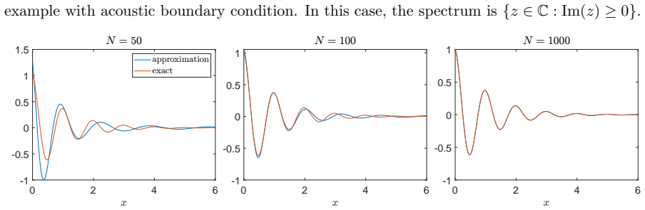
- [§4.3–4.5] Section 4.3 introduces a z-dependent orthonormal basis obtained by Gram-Schmidt and states without proof that 'the convergence results in Section 3.3 continue to hold under this relaxed assumption.' The theorems require a fixed basis whose spans are cores of both T(z) and T(z)*. In the wave-equation example the basis functions do not lie in the domain of T(z), the modified basis depends on z, and no core condition is verified for T(z)*. If the second term of gamma_{n2}(z,T) fails to converge down to gamma(z,T), spectral invisibility can occur. Sections 4.4 and 4.5 also do not verify the core condition for the bases used. Consequently, the differential-operator demonstrations are not consequences of Theorems 3.1 and 3.2 as written. The authors should either provide a proof for a relaxed-core theorem covering their z-dependent and Gram-Schmidt constructions, or explicitly present these examples as numerical demonstrations under an unverified heuristic assumption.
minor comments (4)
- [Throughout] There are several typos, including 'Pseudosepctra' in the caption of Figure 1 and 'the prof if' in the proof of Proposition 3.4.
- [§2.3] The extension of the Attouch-Wets metric to the empty set is described by a convergence convention rather than by an explicit metric. For a fully rigorous SCI formulation, the empty set should be incorporated into the metric space with a defined distance, or the convention should be justified as a limiting metric.
- [References] Several references are incomplete or lack publication details, including [9], [10], [11], [13], [24], [39], and [47]; for example, [9] lists only volume and pages without a journal or article title.
- [§4.1–4.2] The notation for the truncated injection modulus alternates between gamma_{n2}(z,T) and gamma_n(z,T), and in Figure 4 the legend uses both; standardizing this notation would improve readability.
Circularity Check
No significant circularity: the spectral algorithms are derived from an explicit injection-modulus identity with proven convergence, and the cited prior hardness results are independent support rather than an input-output loop.
full rationale
The derivation is self-contained and non-circular. The central reduction is Eq. (3.1), Sp(T)={z in U: gamma(z,T)=0} and Sp_epsilon(T)=Cl_U({z: gamma(z,T)<epsilon}), which follows from Lemma 3.1 proved in the paper (injection modulus equals the inverse norm when boundedly invertible, and min{sigma_inf,sigma_inf*}=0 otherwise). Algorithms 1 and 2 then operate on finite-dimensional singular values gamma_{n2,n1}(z,T) computed from Lambda_1/Lambda_2 matrix elements; the convergence statements in Propositions 3.3 and 3.4 are proved by monotone approximation and continuity of gamma, not by assuming the spectrum. No fitted parameter, calibration set, or predicted quantity is defined in terms of the output, and the output sets are not used as inputs to the algorithm. The lower bounds in Theorem 3.1 and Proposition 3.5 do cite the authors' earlier papers [6], [26], and [28], but those are published, parameter-free hardness theorems for linear and decision problems whose assumptions do not include the nonlinear spectral problem, so they are external support rather than a self-citation loop. The one notable gap is in Section 4.3, where the authors state 'The convergence results in Section 3.3 continue to hold under this relaxed assumption' after introducing z-dependent Gram-Schmidt bases; this is an unproved extension, and Definition 2.4's core condition is an extra hypothesis, but this is a correctness or assumption gap in the examples, not an equivalence between output and input, and it does not make the core derivation circular. Hence no circularity; score 0.
Assumptions & free parameters
assumptions (6)
- standard math Kato's gap-metric theory of closed operators, including generalized convergence and Theorem 2.1 properties.
- domain assumption For each z in U, span{e_n} is a core of T(z) and span{e_hat_n} is a core of T(z)* (Definition 2.4).
- standard math Prior hardness theorems: linear spectrum and pseudospectrum lower bounds of [6, 46] and the Delta^G_3 bound for Xi_{2,Q} of [28].
- domain assumption Dense rational grids G_n with the stated density property (Section 2.4) and exact evaluation of matrix elements at grid points.
- domain assumption Unproved example facts: Sp(T) = {z : Im(z) >= 0} for the acoustic problem (4.3); essential spectrum of H0 is [0,1] union [3,4] for the Klein-Gordon example (4.2).
- ad hoc to paper Convergence of the algorithms extends to z-dependent orthonormal bases built by Gram-Schmidt (Section 4.3).
Cite this review
Pith. "Pith review of Universal Methods for Nonlinear Spectral Problems." pith.science (2026). https://pith.science/paper/X252PWKZ
@misc{pith2026250417012,
  author       = {Pith},
  title        = {Pith review of: Universal Methods for Nonlinear Spectral Problems},
  year         = {2026},
  howpublished = {\url{https://pith.science/paper/X252PWKZ}},
  note         = {Machine review of arXiv:2504.17012}
}
read the original abstract
Nonlinear spectral problems arise across a range of fields, including mechanical vibrations, fluid-solid interactions, and photonic crystals. Discretizing infinite-dimensional nonlinear spectral problems often introduces significant computational challenges, particularly spectral pollution and invisibility, which can distort or obscure the true underlying spectrum. We present the first general, convergent computational method for computing the spectra and pseudospectra of nonlinear spectral problems. Our approach uses new results on nonlinear injection moduli and requires only minimal continuity assumptions: specifically, continuity with respect to the gap metric on operator graphs, making it applicable to a broad class of problems. We use the Solvability Complexity Index (SCI) hierarchy, which has recently been used to resolve the classical linear problem, to systematically classify the computational complexity of nonlinear spectral problems. Our results establish the optimality of the method and reveal that Hermiticity does not necessarily simplify the computational complexity of these nonlinear problems. Comprehensive examples -- including nonlinear shifts, Klein--Gordon equations, wave equations with acoustic boundary conditions, time-fractional beam equations, and biologically inspired delay differential equations -- demonstrate the robustness, accuracy, and broad applicability of our methodology.
Figures


Figures from the paper (9 more)




Reference graph
Works this paper leans on
-
[1]
Adcock and A
B. Adcock and A. C. Hansen. Compressive Imaging: Structure, Sampling, Learning . Cambridge University Press, Cambridge, 2021
2021
-
[2]
Arendt, C
W. Arendt, C. J. K. Batty, M. Hieber, and F. Neubrander. Cauchy Problems. In Vector-valued Laplace Transforms and Cauchy Problems , pages 109–240. Springer Basel, 2001
2001
-
[3]
Baleanu, K
D. Baleanu, K. Diethelm, E. Scalas, and J. J. Trujillo. Fractional calculus: models and numerical methods, volume 3. World Scientific, 2012
2012
-
[4]
A. Bastounis, A. C. Hansen, and V. Vlaˇ ci´ c. The extended Smale’s 9th problem – On computational barriers and paradoxes in estimation, regularisation, computer-assisted proofs and learning. arXiv preprint arXiv:2110.15734, 2021
-
[5]
G. Beer. Topologies on Closed and Closed Convex Sets , volume 268 of Mathematics and its Appli- cations. Springer Netherlands, 1993
1993
-
[6]
J. Ben-Artzi, M. J. Colbrook, A. C. Hansen, O. Nevanlinna, and M. Seidel. Computing spec- tra - On the solvability complexity index hierarchy and towers of algorithms. arXiv preprint arXiv:1508.03280, 2020
arXiv 2020
-
[7]
Ben-Artzi, M
J. Ben-Artzi, M. Marletta, and F. R¨ osler. Computing scattering resonances.Journal of the European Mathematical Society, 25(9):3633–3663, 2022
2022
-
[8]
Ben-Artzi, M
J. Ben-Artzi, M. Marletta, and F. R¨ osler. Computing the sound of the sea in a seashell.Foundations of Computational Mathematics , 22(3):697–731, 2022
2022
Show all 96 references
-
[9]
Betcke, N
T. Betcke, N. J. Higham, V. Mehrmann, C. Schr¨ oder, and F. Tisseur. NLEVP: A collection of nonlinear eigenvalue problems. 39(2):1–28, 2013
2013
-
[10]
Betcke and L
T. Betcke and L. N. Trefethen. Reviving the method of particular solutions. 47(3):469–491, 2005
2005
-
[11]
Bindel and M
D. Bindel and M. Zworski. Theory and computation of resonances in 1d scattering. 2006
2006
-
[12]
L. Blum, F. Cucker, M. Shub, and S. Smale. Complexity and Real Computation . Springer New York, Secaucus, NJ, USA, 1998
1998
-
[13]
Botchev, G
M. Botchev, G. Sleijpen, and A. Sopaheluwakan. An SVD-approach to Jacobi–Davidson solution of nonlinear Helmholtz eigenvalue problems. 431(3-4):427–440, 2009
2009
-
[14]
B¨ ottcher
A. B¨ ottcher. Pseudospectra and singular values of large convolution operators. 6(3):267–301, Sept. 1994
1994
-
[15]
B¨ ottcher
A. B¨ ottcher. Infinite matrices and projection methods. In Lectures on operator theory and its applications (Waterloo, ON, 1994) , volume 3 of Fields Institute Monographs, pages 1–72. American Mathematical Society, 1996
1994
-
[16]
B¨ ottcher and B
A. B¨ ottcher and B. Silbermann. The finite section method for Toeplitz operators on the quarter- plane with piecewise continuous symbols. Math. Nachr., 110:279–291, 1983
1983
-
[17]
B¨ ottcher and B
A. B¨ ottcher and B. Silbermann. Introduction to Large Truncated Toeplitz Matrices . Universitext. Springer-Verlag, New York, 1999
1999
-
[18]
B¨ ottcher and B
A. B¨ ottcher and B. Silbermann. Analysis of Toeplitz Operators . Springer Monographs in Mathe- matics. Springer Berlin Heidelberg, second edition, 2006
2006
-
[19]
B¨ ottcher and I
A. B¨ ottcher and I. M. Spitkovsky. A gentle guide to the basics of two projections theory. Linear Algebra and its Applications , 432(6):1412–1459, 2010
2010
-
[20]
N. P. Brown. AF embeddings and the numerical computation of spectra in irrational rotation algebras. Numerical Functional Analysis and Optimization , 27(5-6):517–528, 2006
2006
-
[21]
N. P. Brown. Invariant means and finite representation theory of C*-algebras. Memoirs of the American Mathematical Society, 184(865), 2006
2006
-
[22]
N. P. Brown. Quasi-diagonality and the finite section method. Mathematics of Computation , 76(257):339–361, 2007. 28
2007
-
[23]
M. Caputo. Linear models of dissipation whose Q is almost frequency independent-II. Geophysical Journal International, 13(5):529–539, 1967
1967
-
[24]
Chaitin-Chatelin and M
F. Chaitin-Chatelin and M. B. van Gijzen. Analysis of parameterized quadratic eigenvalue problems in computational acoustics with homotopic deviation theory. 13(6):487–512, 2006
2006
-
[25]
Chandler-Wilde, R
S. Chandler-Wilde, R. Chonchaiya, and M. Lindner. On spectral inclusion sets and computing the spectra and pseudospectra of bounded linear operators. Journal of Spectral Theory, 14(2):719–804, 2024
2024
-
[26]
M. J. Colbrook. The Foundations of Infinite-dimensional Spectral Computations . PhD thesis, University of Cambridge, 2020
2020
-
[27]
M. J. Colbrook. Computing semigroups with error control. SIAM Journal on Numerical Analysis , 60(1):396–422, 2022
2022
-
[28]
M. J. Colbrook. On the computation of geometric features of spectra of linear operators on Hilbert spaces. Foundations of Computational Mathematics , pages 1–82, 2022
2022
-
[29]
M. J. Colbrook, V. Antun, and A. C. Hansen. The difficulty of computing stable and accurate neural networks: On the barriers of deep learning and Smale’s 18th problem. Proceedings of the National Academy of Sciences , 119(12):e2107151119, 2022
2022
-
[30]
M. J. Colbrook and L. J. Ayton. A contour method for time-fractional PDEs and an application to fractional viscoelastic beam equations. Journal of Computational Physics , 454:110995, 2022
2022
-
[31]
M. J. Colbrook and A. C. Hansen. The foundations of spectral computations via the solvability complexity index hierarchy. Journal of the European Mathematical Society, 25(12):4639–4728, 2022
2022
-
[32]
M. J. Colbrook, I. Mezi´ c, and A. Stepanenko. Limits and powers of Koopman learning. Preprint: arXiv:2407.06312, 2024
2024 arXiv
-
[33]
M. J. Colbrook, B. Roman, and A. C. Hansen. How to compute spectra with error control. Physical Review Letters, 122(25):250201, 2019
2019
-
[34]
M. J. Colbrook and A. Townsend. Avoiding discretization issues for nonlinear eigenvalue problems. SIAM Journal on Matrix Analysis and Applications , 46(1):648–675, 2025
2025
-
[35]
Cordes and J
H. Cordes and J. P. Labrousse. The invariance of the index in the metric space of closed operators. Journal of Mathematics and Mechanics , pages 693–719, 1963
1963
-
[36]
Doyle and C
P. Doyle and C. McMullen. Solving the quintic by iteration. Acta Mathematica, 163(1):151–180, 1989
1989
-
[37]
Dyatlov and M
S. Dyatlov and M. Zworski. Stochastic stability of Pollicott–Ruelle resonances. Nonlinearity, 28(10):3511–3533, 2015
2015
-
[38]
L. B. Eldred, W. P. Baker, and A. N. Palazotto. Kelvin-Voigt versus fractional derivative model as constitutive relations for viscoelastic materials. AIAA Journal, 33(3):547–550, 1995
1995
-
[39]
Engstr¨ om and M
C. Engstr¨ om and M. Wang. Complex dispersion relation calculations with the symmetric interior penalty method. Inter. J. Numer. Meth. Eng. , 84(7):849–863, 2010
2010
-
[40]
W. F. Fagan, R. S. Cantrell, and C. Cosner. How habitat edges change species interactions. The American Naturalist, 153(2):165–182, 1999
1999
-
[41]
T. Faria. Stability and bifurcation for a delayed predator–prey model and the effect of diffusion. Journal of Mathematical Analysis and Applications , 254(2):433–463, 2001
2001
-
[42]
Galkowski and M
J. Galkowski and M. Zworski. Viscosity limits for zeroth-order pseudodifferential operators. Com- munications on Pure and Applied Mathematics , 75(8):1798–1869, 2022
2022
-
[43]
S. A. Gershgorin. Uber die Abgrenzung der Eigenwerte einer Matrix. Izvestija Akademii Nauk SSSR, Serija Matematika , 6:749–754, 1931
1931
-
[44]
I. T. Gokhberg and M. Krein. The basic propositions on defect numbers, root numbers and indices of linear operators. Uspekhi Mat. Nauk , 12(2):43–118, 1957
1957
-
[45]
Guglielmi, M
N. Guglielmi, M. L´ opez-Fern´ andez, and M. Manucci. Pseudospectral roaming contour integral methods for convection-diffusion equations. Journal of Scientific Computing , 89(1):1–31, 2021. 29
2021
-
[46]
A. C. Hansen. On the solvability complexity index, the n-pseudospectrum and approximations of spectra of operators. Journal of the American Mathematical Society , 24(1):81–124, 2011
2011
-
[47]
Harari, K
I. Harari, K. Grosh, T. Hughes, M. Malhotra, P. Pinsky, J. Stewart, and L. Thompson. Recent developments in finite element methods for structural acoustics. Arch. Comput. Meth. Eng. , 3:131– 309, 1996
1996
-
[48]
R. Hilfer. Applications of fractional calculus in physics . World scientific, 2000
2000
-
[49]
Jarlebring
E. Jarlebring. The spectrum of delay-differential equations: Numerical methods, stability and per- turbation. PhD thesis, 2008
2008
-
[50]
T. Kato. Perturbation theory for nullity, deficiency and other quantities of linear operators. Journal d’Analyse Math´ ematique, 6(1):261–322, 1958
1958
-
[51]
T. Kato. Perturbation Theory for Linear Operators, volume 132. Springer Berlin Heidelberg, second edition, 1995
1995
-
[52]
M. G. Krein and M. A. Krasnoselski. Fundamental theorems concerning the extension of Hermitian operators and some of their applications to the theory of orthogonal polynomials and the moment problem. Uspekhi Mat. Nauk. , 2:60–106, 1947
1947
-
[53]
Kukelova, M
Z. Kukelova, M. Bujnak, and T. Pajdla. Polynomial eigenvalue solutions to the 5-pt and 6-pt relative pose problems. In BMVC, volume 2, page 2008, 2008
2008
-
[54]
Lancaster
P. Lancaster. Lambda-matrices and vibrating systems. Courier Corporation, 2002
2002
-
[55]
Langer, B
H. Langer, B. Najman, and C. Tretter. Spectral theory of the Klein–Gordon equation in Pontryagin spaces. Communications in mathematical physics , 267(1):159–180, 2006
2006
-
[56]
Langer, B
H. Langer, B. Najman, and C. Tretter. Spectral theory of the Klein–Gordon equation in Krein spaces. Proceedings of the Edinburgh Mathematical Society, 51(3):711–750, 2008
2008
-
[57]
Laptev and Y
A. Laptev and Y. Safarov. Szeg˝ o type limit theorems. Journal of Functional Analysis , 138(2):544– 559, 1996
1996
-
[58]
Lewandowski and B
R. Lewandowski and B. Chorazyczewski. Identification of the parameters of the Kelvin–Voigt and the Maxwell fractional models, used to modeling of viscoelastic dampers. Computers & Structures , 88(1):1–17, 2010
2010
-
[59]
Li and F
C. Li and F. Zeng. Numerical methods for fractional calculus , volume 24. CRC Press, 2015
2015
-
[60]
B.-S. Liao, Z. Bai, L.-Q. Lee, and K. Ko. Nonlinear Rayleigh–Ritz iterative method for solving large scale nonlinear eigenvalue problems. Taiwanese J. Math., 14(3A):869–883, 2010
2010
-
[61]
Lundberg
L.-E. Lundberg. Spectral and scattering theory for the Klein-Gordon equation. Communications in Mathematical Physics, 31:243–257, 1973
1973
-
[62]
R. L. Magin. Fractional calculus models of complex dynamics in biological tissues. Computers & Mathematics with Applications , 59(5):1586–1593, 2010
2010
-
[63]
Mainardi
F. Mainardi. Fractional calculus and waves in linear viscoelasticity: An introduction to mathematical models. World Scientific, 2010
2010
-
[64]
McLean and V
W. McLean and V. Thom´ ee. Maximum-norm error analysis of a numerical solution via Laplace transformation and quadrature of a fractional-order evolution equation. IMA journal of numerical analysis, 30(1):208–230, 2010
2010
-
[65]
McLean and V
W. McLean and V. Thom´ ee. Numerical solution via Laplace transforms of a fractional order evolu- tion equation. The Journal of Integral Equations and Applications , pages 57–94, 2010
2010
-
[66]
McMullen
C. McMullen. Families of rational maps and iterative root-finding algorithms. Annals of Mathe- matics, 125(3):467–493, 1987
1987
-
[67]
McMullen
C. McMullen. Braiding of the attractor and the failure of iterative algorithms. Inventiones Mathe- maticae, 91(2):259–272, 1988
1988
-
[68]
Mehrmann and C
V. Mehrmann and C. Schr¨ oder. Nonlinear eigenvalue and frequency response problems in industrial practice. J. Math. Ind. , 1:1–18, 2011. 30
2011
-
[69]
Metzler and J
R. Metzler and J. Klafter. The random walk’s guide to anomalous diffusion: A fractional dynamics approach. Physics reports, 339(1):1–77, 2000
2000
-
[70]
D. Mugnolo. Abstract wave equations with acoustic boundary conditions. Mathematische Nachrichten, 279(3):299–318, 2006
2006
-
[71]
Olver and A
S. Olver and A. Townsend. A fast and well-conditioned spectral method. 55(3):462–489, 2013
2013
-
[72]
Olver and A
S. Olver and A. Townsend. A practical framework for infinite-dimensional linear algebra. In 2014 First Workshop for High Performance Technical Computing in Dynamic Languages , HPTCDL ’14, pages 57–62, Piscataway, NJ, USA, 2014. IEEE
2014
-
[73]
Pang and H.-W
H.-K. Pang and H.-W. Sun. Fast numerical contour integral method for fractional diffusion equa- tions. J. Sci. Comput. , 66(1):41–66, 2016
2016
-
[74]
T. Pritz. Five-parameter fractional derivative model for polymeric damping materials. Journal of Sound and Vibration , 265(5):935–952, 2003
2003
-
[75]
R¨ osler and C
F. R¨ osler and C. Tretter. Computing Klein-Gordon spectra. IMA Journal of Numerical Analysis , 2024
2024
-
[76]
J. A. T. M. J. Sabatier, O. P. Agrawal, and J. A. T. Machado. Advances in fractional calculus , volume 4. Springer, 2007
2007
-
[77]
Sakoda, N
K. Sakoda, N. Kawai, T. Ito, A. Chutinan, S. Noda, T. Mitsuyu, and K. Hirao. Photonic bands of metallic systems. I. Principle of calculation and accuracy. Phys. Rev. B , 64(4):045116, 2001
2001
-
[78]
Schiff, H
L. Schiff, H. Snyder, and J. Weinberg. On the existence of stationary states of the mesotron field. Physical Review, 57(4):315, 1940
1940
-
[79]
Schwinger
J. Schwinger. Unitary operator bases. Proceedings of the National Academy of Sciences, 46(4):570– 579, 1960
1960
-
[80]
Shargorodsky
E. Shargorodsky. On the level sets of the resolvent norm of a linear operator. Bulletin of the London Mathematical Society, 40(3):493–504, 2008
2008
-
[81]
Sj¨ ostrand and M
J. Sj¨ ostrand and M. Zworski. Asymptotic distribution of resonances for convex obstacles. Acta Mathematica, 183(2):191–253, 1999
1999
-
[82]
S. Smale. The fundamental theorem of algebra and complexity theory. Bulletin of the American Mathematical Society, 4(1):1–36, 1981
1981
-
[83]
S. Smale. On the efficiency of algorithms of analysis. Bulletin of the American Mathematical Society, 13(2):87–122, 1985
1985
-
[84]
S. Smale. Complexity theory and numerical analysis. Acta Numerica, 6:523–551, 1997
1997
-
[85]
Steinbach and G
O. Steinbach and G. Unger. A boundary element method for the Dirichlet eigenvalue problem of the Laplace operator. 113:281–298, 2009
2009
-
[86]
G. Szeg˝ o. Beitr¨ age zur Theorie der Toeplitzschen Formen.Mathematische Zeitschrift, 6(3-4):167– 202, 1920
1920
-
[87]
L. N. Trefethen and J. A. C. Weideman. The exponentially convergent trapezoidal rule. SIAM Review, 56(3):385–458, 2014
2014
-
[88]
W. Tucker. Validated Numerics. Princeton University Press, 2011
2011
-
[89]
A. M. Turing. On computable numbers, with an application to the Entscheidungsproblem. Pro- ceedings of the London Mathematical Society , s2-42(1):230–265, 1937
1937
-
[90]
H. Voss. A rational spectral problem in fluid-solid vibration. Preprints des Institutes f¨ ur Mathematik, 2002
2002
-
[91]
M. Webb. Isospectral Algorithms, Toeplitz Matrices and Orthogonal Polynomials . PhD thesis, University of Cambridge, 2017
2017
-
[92]
Webb and S
M. Webb and S. Olver. Spectra of Jacobi operators via connection coefficient matrices. 382(2):657– 707, 2021. 31
2021
-
[93]
R. Weder. Scattering theory for the Klein-Gordon equation. Journal of Functional Analysis , 27(1):100–117, 1978
1978
-
[94]
J. A. C. Weideman. Optimizing Talbot’s contours for the inversion of the Laplace transform. SIAM Journal on Numerical Analysis , 44(6):2342–2362, 2006
2006
-
[95]
M. Zworski. Resonances in physics and geometry. Notices of the American Mathematical Society , 46(3):319–328, 1999
1999
-
[96]
M. Zworski. Scattering resonances as viscosity limits. In Algebraic and Analytic Microlocal Analysis, pages 635–654. Springer International Publishing, 2018. 32
2018
Reviewed August 16, 2026 · model on record in the stance chip above.
Discussion (0). Continue with ORCID to comment.