REVIEW 3 major objections 4 minor 66 references
The Magnetic Keys to Massive Star Formation: The Western $\eta$ Carinae Giant Molecular Cloud
T0 review · 3 major / 4 minor · reviewed 2026-08-16 · deepseek-v4-flash
Pith's one-line read This paper argues that magnetic fields provide enough support against gravity to explain the low star formation rate of the massive clumps in the western Eta Carinae molecular cloud, and identifies the column density threshold where…
desk verdict New HAWC+ maps give the field a homogeneous 17-clump sample at one distance, and the subcritical trend is probably real; but the DCF-based mass-to-flux numbers rest on a depth estimate that is uncalibrated and biased exactly where it matters. read the letter →
The pith
A machine-rendered reading of the paper's core claim, the machinery that carries it, and where it could break.
The reading
What carries the argument
The argument is carried by two statistical tools and one geometric estimate. The HRO shape parameter $\xi$ compares the orientation of the magnetic field to the tangent of column-density contours, with $\xi>0$ meaning parallel and $\xi<0$ perpendicular; a linear fit $\xi = C_{\rm HRO}(\log N - X_{\rm HRO})$ locates the critical column density where the field alignment switches. The DCF method converts the dispersion of polarization angles into a plane-of-sky field strength $B_\perp$, and the mass-to-flux ratio $\lambda = 6.38\,(N_{\rm H_2}/10^{26}\,{\rm m^{-2}})/(B_{\rm TOT}/{\rm nT})$ measures whether gravity or magnetism dominates. The geometric estimate is the 'inverse relative gradient' depth $R = N_{\rm H_2}/\nabla N_{\rm H_2}$, used to convert column density into volume density; the paper itself notes this fails near column-density peaks, where it substitutes the projected beam size when the Laplacian is negative. This $R$ value feeds every $B_\perp$ and $\lambda$ map, so it is the main structural assumption in the analysis.
What would settle it
Pick one clump, say BYF68, and obtain an independent line-of-sight depth (for instance, from molecular-line excitation ratios or from the sizes of its embedded cores), then recompute the DCF $B_\perp$ and $\lambda$ maps with those depths instead of the inverse-relative-gradient values. If the resulting mean $\log\lambda$ shifts by more than about 0.3 or moves across the subcritical-to-supercritical boundary, the paper's conclusion is not stable under its depth assumption; if it does not, the assumption is validated for that clump.
Extended reading notes
Core claim
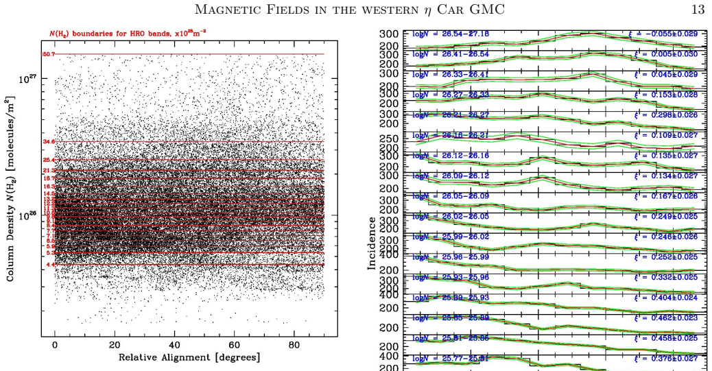
The central claim is that in this sample of parsec-scale massive clumps, magnetic fields are strong enough to hold gravity in check over most of the mapped area, which is why star formation proceeds slowly despite large reservoirs of dense gas. The evidence has two independent legs. Histogram of relative orientation (HRO) analysis shows the expected transition from parallel to perpendicular field alignment with increasing column density, at $N_{\rm crit} = (3.7\pm0.6)\times10^{26}\,{\rm m^{-2}}$ for the whole region and at a similar threshold in the ten 'nominal' clumps; the other seven clumps are exceptions whose fields are controlled by the radiation and overpressure of NGC 3324. Davis\textendash Chandrasekhar\textendash Fermi (DCF) analysis gives field strengths of roughly 10\textendash 200 nT, with a peak of 469 nT, placing the $B$\textendash$n$ data mostly above the Crutcher (2012) relation and giving a mostly subcritical mass-to-flux ratio. The paper also shows that colder dust is statistically much more likely to sit in supercritical gas, linking the magnetic criticality threshold to the known trend of dust temperature falling toward clump centers.
Load-bearing premise
The load-bearing premise is that the line-of-sight depth of the gas, estimated as the inverse relative gradient of the Herschel column-density map ($R = N_{\rm H_2}/\nabla N_{\rm H_2}$, with a beam-size substitution at column-density peaks), is a fair approximation to the true cloud depth; every $B_\perp$ and $\lambda$ map inherits this assumption, and the paper does not calibrate it against any independent depth measurement.
Editorial extensions
If this is right
- If magnetic support is the main brake on star formation, then the low star formation efficiency of the region is not caused by a shortage of dense gas but by the field's resistance to collapse; star formation should be concentrated in the few cold spots where $\lambda$ exceeds 1.
- The high critical column density ($\log N_{\rm crit} = 26.56$) compared with nearer, lower-mass clouds implies that massive clumps can remain magnetically supported up to higher column densities, pushing the onset of collapse to denser, colder gas.
- The split between ten 'nominal' clumps and seven flat or reversed clumps indicates that external feedback from an HII region can locally reset the magnetic field\textendash gravity balance, so environment, not just column density, determines where stars form.
- The temperature trend, with the fraction of pixels having $\log\lambda>0$ rising from 0.08% in the warmest quintile to 12.4% in the coolest, ties the magnetic criticality threshold to dust temperature, consistent with the known $T_{\rm dust}$\textendash$N_{\rm H_2}$ anticorrelation toward clump centers.
- Strong fields ($B>100$ nT) appear in 5% of the high-signal pixels in just a fraction of one GMC, so the 'high-field' part of the $B$\textendash$n$ diagram may be more populated than previously thought, with correspondingly higher critical field strengths for massive star formation.
Reading between the lines
- A testable extension is to use the HRO slope split (nominal vs. flat or reversed) as a diagnostic of external feedback in other clouds near HII regions; the sample here is small, but the pattern is specific enough to look for elsewhere.
- Because $B_\perp \propto n^{1/2}$, a systematic error in the inverse-relative-gradient depth shifts inferred field strengths only weakly, but it shifts $\lambda$ directly; an independent depth calibration for even one clump would show whether the subcritical mean is real.
- The $\log\lambda$\textendash$T_{\rm dust}$ correlation suggests a prediction: at higher angular resolution, the gas that is already supercritical should coincide with the coldest, densest pixels, and the transition should sharpen toward clump centers; this can be checked with ALMA or next-generation far-infrared polarimetry.
- Implicitly, if the critical column density shifts with environment, star-formation efficiency in massive clumps may be regulated by the local radiation field as much as by the magnetic field\textendash gravity balance; comparing $N_{\rm crit}$ in isolated massive clumps with this feedback-affected region would clarify that.
Signed reviews
Editorial analysis
A structured set of objections, weighed in public.
Referee Report
Summary. The paper presents SOFIA/HAWC+ 154 μm polarimetry of 17 massive clumps in Region 9 of the CHaMP survey at the western end of the η Carinae GMC, observed at a fixed physical resolution of 0.16 pc. The authors apply Davis-Chandrasekhar-Fermi (DCF) and Histogram of Relative Orientation (HRO) analyses to map the plane-of-sky magnetic field strength B⊥, the mass-to-flux ratio λ, and the field alignment relative to column-density structures. They report a mostly subcritical cloud (mean log λ = -0.75 ± 0.45 under classical DCF), an HRO transition at log N_crit = 26.56 ± 0.07, and B–n values lying somewhat above the Crutcher (2012) relation. They conclude that magnetic fields provide enough support against gravity to explain the low star formation rate in these massive clumps, except in regions strongly affected by feedback from the HII region NGC 3324.
Significance. If the central quantitative result survives scrutiny, this is a valuable contribution to massive star formation studies: it provides one of the first systematic, fixed-resolution surveys of magnetic support across a single GMC containing clumps in all evolutionary stages. The dataset is substantial (about 9000 independent polarization measurements), the analysis uses two standard and partially independent methods that both indicate the importance of magnetic support, and the authors are commendably explicit about key limitations, including the built-in B–n correlation in DCF and the absence of a direct ξ<0 detection in the HRO data. The HRO transition column is a quantitative, falsifiable prediction that can be tested with Zeeman or higher-resolution polarimetry. However, the quantitative subcritical conclusion rests on an uncalibrated line-of-sight depth estimate that needs a sensitivity analysis before the results can be fully trusted.
major comments (3)
- [§3.1, Eq. (3)] The IRG-based depth estimate is the load-bearing input for all quantitative DCF results, but it is never calibrated against an independent measure of cloud depth. Because B⊥ ∝ sqrt(N/R) (Eq. 1) and λ ∝ N/B_TOT ∝ sqrt(N R) (Eq. 4), capping R at the 0.16 pc beam wherever the Laplacian is negative suppresses λ near column-density peaks by roughly sqrt(0.16/R_true), i.e., about 0.4 dex for a typical clump depth of 1 pc, and more for larger clumps. This bias acts exactly in the regions where gravity is expected to dominate, so the reported mean log λ = -0.75 and the statement that 'only small areas are dominated by gravity' may be substantially in error. I recommend (a) validating the IRG-derived R against independent depth estimates for at least a subset of clumps (e.g., sizes from the Mopra 12CO ellipses, or column-density/volume-density comparisons), and (b) recomputing the λ maps and the supercritical fraction under a range of plausible R assumptions (e.g., constant R per clump, R = projected diameter, or a factor 2–3 larger near peaks) to demonstrate the robustness of the subcritical conclusion.
- [§3.2 and Abstract] The quoted threshold log N_crit = 26.56 ± 0.07 is the zero-crossing of a linear fit to the HRO shape parameter ξ(N), but the text explicitly states that the data 'do not clearly progress to a column density regime where the alignments are more perpendicular (i.e., ξ < 0)'. The crossing point is therefore an extrapolation beyond the range of directly sampled ξ values (the highest bins have ξ consistent with zero, not negative). The abstract's claim that the threshold 'indicat[es] that gravitational forces exceed magnetic forces above this value' overstates the direct evidence. Please rephrase the claim to reflect that the data show a strong trend toward criticality at this column density, with the actual crossing being an extrapolation, and consider reporting the column density at which ξ becomes consistent with zero at the 1σ level rather than the formal zero-crossing.
- [§3.3, Figure 16 and surrounding text] The B–n diagram analysis compares the fitted slope κ ≈ 0.5 to the Crutcher (2012) relation, but this slope is largely built into the construction: from Eq. (1) with n = N/R, B⊥ ∝ sqrt(n) at fixed s and ΔV, so the expected κ is 0.5 regardless of the actual physics. The authors correctly acknowledge this via Pattle et al. (2022) and present the Alfvén number as an alternative, but they still use the vertical offset ('a factor of ~2.5 above the Crutcher line') to infer 'somewhat higher than typical' field strengths. This offset is the only physically meaningful signal, and it depends directly on the assumed values of Q, L_corr, and R. Please provide a quantitative decomposition: how much of the offset is due to the chosen Q=0.5 and B_TOT=2B⊥ assumptions, and how much survives if R is varied as in the sensitivity analysis above? Without this, the comparison to Crutcher (2012) is difficult to interpret.
minor comments (4)
- [Eq. (3)] The chain of equalities in Eq. (3) is visually confusing because n is written both as N_H2/R and as ∇N_H2; please rewrite to show the two branches separately (one for ∇²N_H2 > 0, one for ∇²N_H2 ≤ 0).
- [§3.3] The text refers to 'the other 7 ROIs' as a single group, but BYF70aN is subsequently described as a separate outlier; please clarify the grouping, e.g., '6 flat ROIs plus 1 outlier, BYF70aN'.
- [Figure 16] The figure label reports χ² = 0.59 for the binned fit; please specify whether this is the reduced chi-squared and state the number of degrees of freedom.
- [Table 1] The t-statistics use sample sizes divided by 2.5² to account for oversampling, but the λ values are spatially correlated on the DCF correlation scale; a more conservative estimate using the number of independent resolution elements would strengthen the significance claim.
Circularity Check
No significant circularity: the central claims are direct measurements from the polarization and column-density data under stated assumptions; the built-in B–n correlation is explicitly acknowledged and reinterpreted as an Alfvén-number diagnostic.
full rationale
The paper's core results—the HRO transition at log Ncrit ≈ 26.56 and the subcritical log λ distribution—are not fitted outputs that reduce to their inputs by construction. The HRO analysis measures the relative angle between the HAWC+ polarization position angles and the Herschel column-density gradients; the ξ(N) trend and its zero crossing are summary statistics of those data, and the data could in principle have shown any slope or crossing. The DCF-derived λ map is computed from explicit formulae (Eqs. 1, 3, 4) using observed N, ΔV, and s, with the line-of-sight depth R estimated by the inverse relative gradient. R is an observational assumption that can bias absolute B and λ, but it is not defined in terms of B or λ, and nothing is calibrated to force the subcritical conclusion. The potentially circular B–n correlation is disclosed: the authors quote Pattle et al. (2022) and state that 'the trends in the Bn diagram are somewhat built-in, since with DCF measurements, B and n are not independent', then reinterpret Figure 16 as the Alfvén number M_A in Figure 17. Thus the paper does not present the B–n slope as an independent prediction. Self-citations to Barnes et al. (2015, 2018, 2023) and Pitts et al. (2019) supply standard methodology and prior observational maps (N_H2, T_dust, ΔV), not an unverified theorem that forces the conclusion; these inputs are external to the new HAWC+ data and could disagree with them. The 'Ncrit' values are fitted zero crossings of the HRO ξ–N regressions, which is a normal way to report a measured threshold rather than a fitted input renamed as a prediction. Overall, the derivation chain is self-contained in the sense that every quantitative claim is traceable to stated equations and data, with the acknowledged built-in correlation handled openly; remaining concerns about the IRG depth estimate are assumption/robustness issues, not circularity.
Assumptions & free parameters
free parameters (3)
- DCF correlation length for angle dispersion, L_corr =
0.33 pc
- DCF correction factor Q =
0.5
- B_total to B_perp ratio in mass-to-flux calculation =
2 (assumed)
assumptions (5)
- domain assumption Far-infrared polarization from aligned dust grains traces the plane-of-sky magnetic field orientation (RAT alignment).
- domain assumption The DCF relation (Eq. 1) and its Skalidis-Tassis variant (Eq. 2) convert the dispersion in polarization angles into a magnetic field strength.
- domain assumption The HRO transition from parallel to perpendicular alignment at a threshold column density indicates the density where gravitational forces overtake magnetic support.
- ad hoc to paper The line-of-sight depth R can be estimated as the inverse relative gradient of the column density map, with a beam-size cap where the Laplacian is negative.
- domain assumption The Mopra N12CO velocity dispersion map at 37 arcsec resolution is representative of the velocity dispersion on HAWC+ 13.6 arcsec scales.
Cite this review
Pith. "Pith review of The Magnetic Keys to Massive Star Formation: The Western $\eta$ Carinae Giant Molecular Cloud." pith.science (2026). https://pith.science/paper/R3ZRIM5D
@misc{pith2026250417842,
  author       = {Pith},
  title        = {Pith review of: The Magnetic Keys to Massive Star Formation: The Western $\eta$ Carinae Giant Molecular Cloud},
  year         = {2026},
  howpublished = {\url{https://pith.science/paper/R3ZRIM5D}},
  note         = {Machine review of arXiv:2504.17842}
}
abstract
We present SOFIA/HAWC+ continuum polarisation data on the magnetic fields threading 17 pc-scale massive molecular clumps at the western end of the $\eta$ Car GMC (Region 9 of CHaMP, representing all stages of star formation from pre-stellar to dispersing via feedback), revealing important details about the field morphology and role in the gas structures of this clump sample. We performed Davis-Chandrasekhar-Fermi and Histogram of Relative Orientation analyses tracing column densities 25.0 $<$ log($N$/m$^{-2}$) $<$ 27.2. With HRO, magnetic fields change from mostly parallel to column density structures to mostly perpendicular at a threshold $N_{\rm crit}$ = (3.7$\pm$0.6)$\times$10$^{26}$ m$^{-2}$, indicating that gravitational forces exceed magnetic forces above this value. The same analysis in 10 individual clumps gives similar results, with the same clear trend in field alignments and a threshold $N_{\rm crit}$ = (1.9$^{+1.5}_{-0.8}$)$\times$10$^{26}$ m$^{-2}$. In the other 7 clumps, the alignment trend with $N$ is much flatter or even reversed, inconsistent with the usual HRO pattern. Instead, these clumps' fields reflect external environmental forces, such as from the nearby HII region NGC 3324. DCF analysis reveals field strengths somewhat higher than typical of nearby clouds, with the $Bn$ data lying mostly above the Crutcher (2012) relation. The mass:flux ratio $\lambda$ across all clumps has a gaussian distribution, with log$\lambda_{\rm DCF}$ = -0.75$\pm$0.45 (mean$\pm\sigma$): only small areas are dominated by gravity. However, a significant trend of rising log$\lambda$ with falling $T_{\rm dust}$ parallels Pitts et al's (2019) result: $T_{\rm dust}$ falls as $N_{\rm H_2}$ rises towards clump centres. Thus, in this massive clump sample, magnetic fields provide enough support against gravity to explain their overall low star formation rate.
Figures


Figures from the paper (13 more)




Reference graph
Works this paper leans on
-
[1]
Andersen, M., Barnes, P. J., Tan, J. C., Kainulainen, J., & G. de Marchi, G. 2017, , 850, 12
work page 2017
-
[2]
Barnes, P. J., Yonekura, Y., Ryder, S. D., et al. 2010, , 402, 73
work page 2010
-
[3]
Barnes, P. J., Yonekura, Y., Fukui, Y. et al. 2011, , 196, 12
work page 2011
-
[4]
Barnes, P. J., Ryder, S. D., O'Dougherty, S. N., et al. 2013, , 432, 2231
work page 2013
-
[5]
J., Li, D., Telesco, C., et al
Barnes, P. J., Li, D., Telesco, C., et al. 2015, , 453, 2622
work page 2015
-
[6]
J., Muller, E., Indermuehle, B., et al
Barnes, P. J., Muller, E., Indermuehle, B., et al. 2015, ,812,6
work page 2015
-
[7]
Barnes, P. J., Hernandez, A. K., O'Dougherty, S. D., Schap, W. J. III, & Muller, E. 2016, , 831, 67
work page 2016
-
[8]
Barnes, P. J., Hernandez, A. K., Muller, E., & Pitts, R. L. 2018, , 866, 19
work page 2018
Show all 66 references
-
[9]
J., Ryder, S
Barnes, P. J., Ryder, S. D., Novak, G., Crutcher, R. M., Fissel, L. M., Pitts, R. L., & Schap, W. J. III 2023, , 945, 34
2023
-
[10]
& Leedom, L
Cabral, B. & Leedom, L. C., 1993, ``Imaging Vector Fields Using Line Integral Convolution,'' Proc. 20th ann. conf. Computer graphics and interactive techniques (SIGGRAPH '93: Anaheim, CA), pp.\ 263--270
1993
-
[11]
1953, , 118, 113
Chandrasekhar, S., & Fermi, E. 1953, , 118, 113
1953
-
[12]
K., & Li, Z.-Y
Chen, C.-Y., King, P. K., & Li, Z.-Y. 2016, , 829, 84
2016
-
[13]
C., Girart, J
Cortes, P. C., Girart, J. M., Sanhueza, P., et al 2024, \ submitted, arXiv:2406.14663
2024 arXiv
-
[14]
M., Nutter, D
Crutcher, R. M., Nutter, D. J., Ward-Thompson, D. & Kirk, J. M. 2004, ApJ, 600, 279
2004
-
[15]
Crutcher, R. M. 2012, , 50, 29
2012
-
[16]
1951, Phys.Rev., 81, 890
Davis, L. 1951, Phys.Rev., 81, 890
1951
-
[17]
H., Crutcher, R
Falgarone, E., Troland, T. H., Crutcher, R. M., & Paubert, G. 2008, A&A, 487, 247
2008
-
[18]
M., Ade, P
Fissel, L. M., Ade, P. A. R., Angil\`e, F. E., et al. 2016, , 824, 134
2016
-
[19]
M., Ade, P
Fissel, L. M., Ade, P. A. R., Angil\`e, F. E., et al. 2019, , 878, 110
2019
-
[20]
1990, , 349, 126
Franco, J., Tenorio-Tagle, G., Bodenheimer, P. 1990, , 349, 126
1990
-
[21]
M., Greaves, J
Girart, J. M., Greaves, J. S., Crutcher, R. M., & Lai, S.-P. 2004, Ap.SpaceSci. 292, 119
2004
-
[22]
& Kylafis N
Goldreich P. & Kylafis N. 1981, , 243, L75
1981
-
[23]
1997, Proc
Gooch, R.\ E. 1997, Proc. Astr. Soc. Aust., 14, 106
1997
-
[24]
J., Cram, L
Green, A. J., Cram, L. E., Large, M. I., & Ye, T. 1999, , 122, 207
1999
-
[25]
Habing, H. J. & Israel, F. P. 1979, , 17, 345
1979
-
[26]
& Crutcher, R
Hakobian, N. & Crutcher, R. 2011, , 733, 6
2011
-
[27]
A., Runyan, M
Harper, D. A., Runyan, M. C., Dowell, C. D., et al. 2018, J.\,Astr.\,Instrum. , 7(4), 184008
2018
-
[28]
M., Koerner D
Howard E. M., Koerner D. W., Pipher J. L., 1997, , 477, 738
1997
-
[29]
2021, Nat.Astron., doi:10.1038/s41550-021-01414z
Jiang, C., et al. 2021, Nat.Astron., doi:10.1038/s41550-021-01414z
2021 doi
-
[30]
Lada, C. J. 2015, in Proc IAU Symposium 309, Galaxies in 3D across the Universe , B Ziegler et al. eds, p31
2015
-
[31]
2007, JQSRT, 106, 225
Lazarian, A. 2007, JQSRT, 106, 225
2007
-
[32]
& Hoang, T
Lazarian, A. & Hoang, T. 2014, 40th COSPAR Scientific Assembly, Abstract F3.2-4-14, http://adsabs.harvard.edu/abs/ 2014cosp...40E1761L
2014
-
[33]
H., Ho, K
Lazarian A., Yuen K. H., Ho, K. W., et al. 2018, , 865, 46
2018
-
[34]
G., Reipurth, B., Ostriker, E
Lee, C-F., Mundy, L. G., Reipurth, B., Ostriker, E. C., & Stone, J. M. 2000, , 542, 925
2000
-
[35]
2021, , 918, 39
Lee, D., Berthoud, M., Chen, C-Y., et al. 2021, , 918, 39
2021
-
[36]
Liu, J., Zhang, Q., Qiu, K., 2022, Front.\ Ast.\ Space Sci., 9, 943556
2022
-
[37]
& Monger, P
Lupton, R. & Monger, P. 2000, SuperMongo Manual, unpublished
2000
-
[38]
& Ostriker, E
McKee, C. & Ostriker, E. 2007, , 45, 565
2007
-
[39]
Mezger, P. G. & Henderson, A. P. 1967, , 147, 471
1967
-
[40]
G., Schraml, J., & Terzian, Y
Mezger, P. G., Schraml, J., & Terzian, Y. 1967, , 150, 807
1967
-
[41]
Ch., & Ciolek, G
Mouschovias, T. Ch., & Ciolek, G. E. 1999, in The Origin of Stars and Planetary Systems , ed. C.J. Lada, N.D. Kylafis, p. 305. Dordrecht: Kluwer
1999
-
[42]
C., & Goodman, A
Myers, P. C., & Goodman, A. A. 1991, , 373, 509
1991
-
[43]
L., Dowell, C
Novak, G., Dotson, J. L., Dowell, C. D., Goldsmith, P. F., Hildebrand, R. H., Platt, S. R., & Schleuning, D. A. 1997, , 487, 320
1997
-
[44]
C., Stone, J
Ostriker, E. C., Stone, J. M., & Gammie, C. F., 2001, , 546, 980
2001
-
[45]
Ouyed, R., & Pudritz, R. E. 1997, , 482, 712
1997
-
[46]
1973, , 78, 929
Panagia, N. 1973, , 78, 929
1973
-
[47]
(arXiv:2203.11179)
Pattle, K., Fissel, L., Tahani, M., Liu, T., & Ntormousi, E.\ 2022, to be published in Protostars and Planets VII , S.-I.\ Inutsuka et al., eds. (arXiv:2203.11179)
2022 arXiv
-
[48]
L., Barnes, P
Pitts, R. L., Barnes, P. J., Ryder, S. D, & Li, D. 2018, , 867, L7
2018
-
[49]
L., Barnes, P
Pitts, R. L., Barnes, P. J., & Varosi, F. 2019, , 484, 305
2019
-
[50]
L., & Barnes, P
Pitts, R. L., & Barnes, P. J. 2021, , 256, 3
2021
-
[51]
Planck Collaboration XXXV 2016, A&A, 586, A138
2016
-
[52]
E., & Ray, T
Pudritz, R. E., & Ray, T. P. 2019, Front.Astron.SpaceSci., 6, 54
2019
-
[53]
C., Canto, J., Calvet, N., Rodr\'iguez, L
Raga, A. C., Canto, J., Calvet, N., Rodr\'iguez, L. F., & Torrelles, J. M. 1993, A&A, 276, 539
1993
-
[54]
H., Bosma, A., van der Hulst, J
Rots, A. H., Bosma, A., van der Hulst, J. M., Athanassoula, E., & Crane, P. C. 1990, , 100, 387
1990
-
[55]
Rygl, K. L. J., Wyrowski, F., Schuller, F., & Menten, K. M. 2013, A&A, 549, 5
2013
-
[56]
Samson, W. B. 2021, J.Br.Astron.Assoc., 131(2), 97
2021
-
[57]
P., Chuss, D
Santos, F. P., Chuss, D. T., Dowell, C. D.,
-
[58]
J., Teuben, P
Sault, R. J., Teuben, P. J., & Wright, M. C. H., 1995. in ``Astronomical Data Analysis Software and Systems IV,'' eds. R. Shaw, H. E. Payne, J. J. E. Hayes, ASP Conference Series, 77, 433
1995
-
[59]
2019, M.Sc
Sharpe, M. 2019, M.Sc. Thesis, University of New England, unpublished
2019
-
[60]
1994, , 429, 781
Shu, F.H., Najita, J., Ostriker, E., Wilkin, F., Ruden, S., & Lizano, S. 1994, , 429, 781
1994
-
[61]
& Tassis, K., 2021, A&A, 647, A186
Skalidis, R. & Tassis, K., 2021, A&A, 647, A186
2021
-
[62]
2017, A&A, 603, A64
Soler, J., Ade, P., Angil\`e, F., et al. 2017, A&A, 603, A64
2017
-
[63]
M., King, P
Sullivan, C., Fissel, L. M., King, P. K., Chen, C.-Y., Li, Z.-Y., & Soler, J. D. 2021, , 503, 5006
2021
-
[64]
2011, PASJ, 63, 147
Tomisaka, K. 2011, PASJ, 63, 147
2011
-
[65]
Whitworth, D.\ J., Srinivasan, S., Pudritz, R.\ E., et al.\ 2024, , submitted (arXiv:2407.18293)
2024 arXiv
-
[66]
S., Schlafly, E
Zucker, C., Speagle, J. S., Schlafly, E. F., Green, G. M., Finkbeiner, D. P., Goodman, A., & Alves, J. 2021, A&A, 633, 51
2021
Reviewed August 16, 2026 · model on record in the stance chip above.
Discussion (0). Continue with ORCID to comment.