REVIEW 5 major objections 7 minor 1 cited by
Schr\"odingerization based quantum algorithms for the fractional Poisson equation
T0 review · 5 major / 7 minor · reviewed 2026-08-16 · deepseek-v4-flash
Pith's one-line read The paper claims a quantum algorithm for the FEM-discretized fractional Poisson equation with query cost Õ(d 3^{3d/2} h^{-2.5}), independent of dimension in the mesh size, an exponential advantage over classical conjugate gradients in…
desk verdict A legitimate new combination with a real gap: the advertised h^{-2.5} complexity rests on an unconstructed VTAA step that the authors themselves flag as open; the paper's own un-amplified bound still delivers the qualitative exponential advantage. read the letter →
The pith
A machine-rendered reading of the paper's core claim, the machinery that carries it, and where it could break.
The reading
What carries the argument
The carrying mechanism is the pairing of the Caffarelli–Silvestre extension with the Schrödingerization transformation. The extension is the identity $d_s(-\Delta)^s u = -\lim_{y\to 0^+} y^{\alpha}u_y$ for $\alpha=1-2s$, realized as the Dirichlet-to-Neumann map of the weighted elliptic equation $\mathrm{div}(y^{\alpha}\nabla u)=0$ on $\Omega\times(0,\infty)$; it replaces the nonlocal operator by a local problem in $d+1$ dimensions. Schrödingerization is the warped-phase change of variables $v(t,p)=e^{-p}u_f(t)$ that sends the dissipative ODE system $du_f/dt = A_f u_f$ into the Schrödinger-type system $\partial_t v = -H_1\partial_p v + iH_2 v$, whose Fourier discretization in the auxiliary variable $p$ is a Hamiltonian system suitable for quantum simulation. The final ingredient is the block-encoding of $A$ as a sum of Kronecker products $A^{(1)}\otimes S^{(2)}\otimes\cdots\otimes S^{(d+1)}$ plus cyclic permutations, which keeps the input-model cost quadratic in $d$ rather than exponential.
What would settle it
Implement the proposed pipeline for a fixed dimension, say $d=2$ or $d=3$, on the FEM-discretized fractional Poisson equation over a sequence of mesh sizes $h$, and count block-encoding queries needed to prepare an $\epsilon$-accurate solution with success probability $\Omega(1)$. If the empirical exponent of $h^{-1}$ exceeds $2.5$, or if the success probability decays polynomially in $h$, the claimed dimension-independent advantage fails; a direct check of Lemma 2.1 against a stiff positive-definite matrix would settle the same question.
Extended reading notes
Core claim
The paper's central claim is that a nonlocal fractional problem can be solved through the local extension it inherits. After truncating the Caffarelli–Silvestre cylinder to $C_Y$ and using tensor-product piecewise-linear finite elements on graded meshes, the stiffness matrix $A$ has sparsity $3^{d+1}$ and condition number $\kappa(A)=O((d+1)3^{d+1}h^{-2})$, and it can be block-encoded as a sum of Kronecker products of one-dimensional stiffness and mass matrices, so the exponentially large sparse matrix is never formed explicitly. Treating $Ax=b$ as the steady state of $du/dt=-Au+b$ and applying Schrödingerization produces a Hamiltonian system whose simulation gives an $\epsilon$-approximation of $|x\rangle$; combining the query bound with the trace projection onto the $y=0$ boundary and amplitude amplification yields the headline $\widetilde{\mathcal{O}}(d 3^{3d/2} h^{-2.5})$ query complexity. Without the variable-time amplitude amplification described in Remark 2.2, the paper's own estimate is $\widetilde{\mathcal{O}}(d^2 3^{5d/2} h^{-4.5})$, still independent of $d$ in the $h^{-1}$ factor.
Load-bearing premise
The load-bearing premise is Lemma 2.1, the query-complexity estimate for the Schrödingerization-based linear-system solver, which the paper states as following 'with some modifications' from another work without proof, together with the variable-time amplitude amplification of Remark 2.2 that is invoked to reach the improved exponent but is explicitly not constructed; if either is unsound, the claimed $\widetilde{\mathcal{O}}(h^{-2.5})$ scaling gives way to the paper's own weaker $\widetilde{\mathcal{O}}(d^2 3^{5d/2}h^{-4.5})$ bound.
Editorial extensions
If this is right
- If the central claim is correct, the fractional Poisson equation loses the classical curse of dimensionality: for fixed mesh size the quantum cost is independent of $d$ in the $h^{-1}$ factor, while classical conjugate gradients scale as $h^{-d-2}$.
- The Kronecker-product block-encoding construction means the $3^{d+1}$-sparse FEM matrix never needs to be assembled or queried entrywise; block-encodings of one-dimensional stiffness and mass matrices suffice.
- The same extension-plus-Schrödingerization pipeline is applied to a finite-difference discretization and to the nonlocal variational formulation, with Remark 5.1 observing that block-encoding of the dense nonlocal matrix remains possible on regular domains.
- Even in the un-amplified version, the cost $\widetilde{\mathcal{O}}(d^2 3^{5d/2}h^{-4.5})$ is still dimension-independent in $h^{-1}$, so the quantum approach would avoid the exponential-in-$d$ mesh dependence even without variable-time amplitude amplification.
- The explicit ingredients $\kappa(A)=O((d+1)3^{d+1}h^{-2})$ and $g=O(3^{d/2}h^{-1/2})$ for the trace projection are what combine into the reported $3^{3d/2}h^{-2.5}$ exponent.
Reading between the lines
- Editorial inference: the same localization-plus-Schrödingerization template could be applied to other nonlocal operators admitting a local extension, such as fractional Laplacians with Neumann or Robin boundary conditions or regional fractional operators, but the paper does not treat those cases.
- Editorial inference: the trace projection is a natural bottleneck, since the cost carries a $3^{d/2}$ factor from recovering the $d$-dimensional solution from the $d+1$-dimensional one; a block-encoding of the trace operator that avoids measurement-and-amplify could improve the dimension dependence.
- Editorial inference: because the headline bound rests on an unproved lemma and an unconstructed subroutine, a direct proof or a numerical query-count test of Lemma 2.1 on stiff FEM matrices is the minimal next step that would make the exponential-advantage claim conclusive.
Signed reviews
Editorial analysis
A structured set of objections, weighed in public.
Referee Report
Summary. The paper proposes a quantum algorithm for the fractional Poisson equation on bounded domains. It first applies the Caffarelli–Silvestre extension to rewrite the nonlocal fractional Laplacian as a local degenerate/singular elliptic problem in one higher dimension, discretizes the resulting problem with a tensor-product finite element method, and then solves the resulting linear system Au=b by interpreting the solution as the steady state of the ODE du/dt=-Au+b and applying the Schrödingerization technique. The main claimed result is a query complexity of Õ(d3^{3d/2}h^{-2.5}) against block-encoding input models, to be compared with a classical conjugate-gradient cost of Õ(d^{1/2}3^{3d/2}h^{-d-2}), giving an exponential quantum advantage in the spatial dimension d for fixed mesh size h. Numerical experiments in one and two dimensions for both the extension formulation and a nonlocal variational formulation are reported.
Significance. If fully established, an exponential quantum advantage in d for a fractional PDE would be a significant result. The combination of the Caffarelli–Silvestre extension with Schrödingerization is natural and potentially impactful, and the manuscript contains genuinely useful components: a transparent block-encoding construction for the FEM stiffness matrix, an explicit trace-extraction step, and numerical validation of the formulation. I also credit the authors for explicitly stating the un-amplified bound Õ(d^2 3^{5d/2}h^{-4.5}) at the end of Section 4.3; even at that bound, the h-dependence remains dimension-independent, so the qualitative exponential advantage may well survive. However, the headline h^{-2.5} bound depends on an essentially unproved lemma and on a VTAA procedure that the authors themselves describe as an open question, and several supporting estimates are incompletely justified. These gaps are load-bearing for the main complexity claim and must be closed before the result can be accepted as stated.
major comments (5)
- [Theorem 4.1 and abstract] The claimed query complexity Õ(d3^{3d/2}h^{-2.5}) in Theorem 4.1 and the abstract is not established. The proof consists of the sentence 'combining Theorem 2.1, the VTAA procedure (see Remark 2.2), Theorem 3.1 and Eq. (4.5)', but Remark 2.2 states that a simple approach to reducing the κ-dependence from quadratic to near-linear remains an open question and that VTAA requires substantial modifications to LCU or QSP algorithms. No VTAA schedule is constructed and no VTAA query count is provided. The paper's own un-amplified bound is Õ(d^2 3^{5d/2}h^{-4.5}) (end of Section 4.3). Please either construct and analyze the VTAA step explicitly, or remove h^{-2.5} from the abstract and Theorem 4.1 and present the un-amplified bound as the main result.
- [Lemma 2.1 and Theorem 2.1] Lemma 2.1 is the foundation of Theorem 2.1 but is not proved in this manuscript; it is introduced with 'Following the similar implementation in [36] with some modifications'. Since [36] is the authors' own concurrent work and the parameter dependence in Lemma 2.1, especially the claim η_max = O(log(1/ε)), is crucial for the final complexity, a self-contained proof or a precise statement of the relevant theorem in [36] is needed. Without this, the query-complexity chain lacks a verified base.
- [Theorem 3.1] The proof of the condition-number estimate treats only the case 0<s<1/2 (0<α<1) and asserts that s>1/2 'can be deduced in a similar manner'. This is not immediate because for α=1-2s<0 the weight y^α is singular at y=0, and the use of the second integral mean-value theorem to extract Y^α is not justified for a singular weight. In addition, the mesh in the extended direction is graded as in (3.9), not quasi-uniform; the quoted bound λ_min(G_ξ) ≳ (h/3)^{d+1} from [25] may not hold for the actual graded mesh. Since κ(A) enters the quantum complexity bound, a complete proof of Theorem 3.1 for all s∈(0,1) and for the graded mesh used by the algorithm is required.
- [Lemma 4.1] The proof of Lemma 4.1 is incomplete. For the 'second inequality' involving S(d+1), the text says only that one can apply the second integral mean-value theorem 'as done in Theorem 3.1', but S(d+1) is a weighted mass matrix and for α<0 the weight is singular, so the asserted bound h/3 ≲ λ(S(d+1)) ≲ h needs a derivation. Moreover, the conclusion g = O(3^{d/2}h^{-1/2}) requires a bound on ∥(uY)_h∥_{L2}/∥u_h∥_{L2}; this trace ratio is not obviously O(1) in the graded-mesh setting and is not discussed. An extra factor here would change the trace-extraction overhead in the final complexity.
- [Section 4.1] The block-encoding construction for A is described at the level of combining univariate block-encodings, but the query cost of constructing the block-encoding oracle for A is not quantified. The sentence 'the complexity of block-encoding A ... has only a quadratic dependence on d' is not accompanied by a count. Since Theorem 4.1 counts queries to the block-encoding oracle of A, the cost of implementing that oracle via the proposed LCU of tensor products must either be included in the total cost or stated as a separate input-model assumption. Without this, the claimed d-dependence of the quantum algorithm is not fully established.
minor comments (7)
- [Section 3.3] In the paragraph following (3.6), 'the the Dirichlet boundary' should read 'the Dirichlet boundary'.
- [Throughout] The spelling of Schrödingerisation/Schrödingerization is inconsistent; please choose one convention and use it consistently.
- [References] References [2] and [3] appear to be the same paper with different years; please merge or correct the entries.
- [Equation (4.4)] The notation 'ui1,···,id,id+1=0' is ambiguous; it should read 'ui1,...,id,0' or clearly set i_{d+1}=0.
- [Lemma 2.1] The condition that the coefficient matrix is 'negative semi-definite over the interval [0,T]' is unclear as stated; if the authors mean that -A in (2.1) is negative definite for positive definite A, the wording should be made precise.
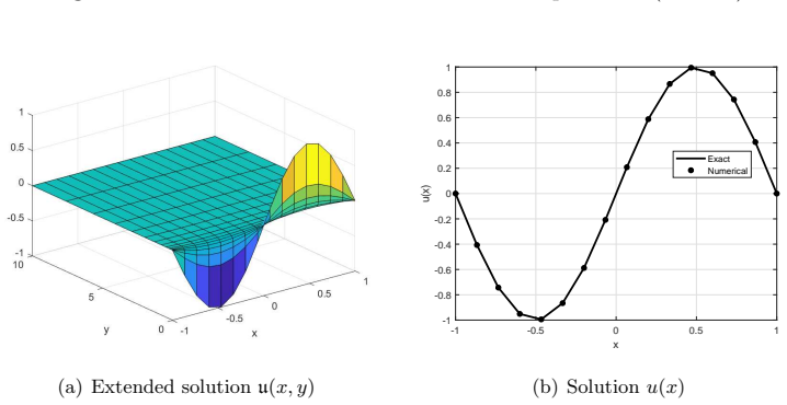
- [Figure 6] The caption of Figure 6 refers to a fixed point (x1,x2)=(0,0) but the example is one-dimensional; please adjust the caption to match the plotted quantity.
- [Abstract] The phrase 'which can show up to exponential advantage' is awkward; consider rewording to 'which yields an exponential advantage'.
Circularity Check
No definitional or fitted-input circularity: the advertised h^{-2.5} query count is not forced by construction, but the proof depends on same-author lemmas and an unconstructed variable-time amplitude amplification step, so the self-citation burden is non-negligible.
full rationale
The derivation is not circular in the strict sense. The Caffarelli-Silvestre extension and its FEM error estimates are taken from external theory (Nochetto et al. [47]), and the new block-encoding construction for the tensor-product stiffness matrix and the trace-projection factor g = O(3^{d/2} h^{-1/2}) are derived in Sections 4.1-4.2 rather than fitted to the desired answer. No parameter is tuned on the fractional Poisson solution to make the h-exponent match a preconceived value. The Schrödingerization framework is imported from the authors' own prior work ([29,36,39,40]), but it is applied as a subroutine to the linear system (3.10); applying a previously developed solver is not a definitional circularity. The main caveat is not circularity: Lemma 2.1 is stated without proof ('Following the similar implementation in [36] with some modifications'), and Remark 2.2 explicitly says the VTAA needed to turn the quadratic kappa-dependence into near-linear 'requires substantial modifications' and that a simple approach 'remains an open question'. Theorem 4.1 nevertheless states the h^{-2.5} bound by combining Theorem 2.1 with that unconstructed VTAA. That is a missing-support/completeness gap, not a fitted input or self-definitional reduction. The un-amplified bound eO(d^2 3^{5d/2} h^{-4.5}) stated in Section 4.3 is the only complexity actually derived from the displayed equations. Because the only circularity-adjacent feature is reuse of same-author lemmas without independent proof, the score is kept at the low end.
Assumptions & free parameters
free parameters (3)
- Evolution time T =
15 (numerical experiments)
- Truncated cylinder height Y =
10 (numerical experiments)
- Number of Fourier modes Np =
2^11 (numerical experiments)
assumptions (6)
- domain assumption Caffarelli-Silvestre extension: the fractional Laplacian is the Dirichlet-to-Neumann map of a degenerate elliptic problem in one higher dimension.
- domain assumption Exponential decay of the extension solution in the extended variable y (Lemma 3.3).
- domain assumption FEM error estimates for graded meshes (Lemma 3.4).
- standard math Eigenvalue bounds for standard FEM matrices (λmax(G)≲(d+1)h^{d-1}, λmin(G_ξ)≳(h/3)^{d+1}).
- domain assumption Schrödingerization convergence and complexity theorems from the authors' prior work (Lemma 2.1, Theorem 2.1).
- standard math Block-encoding and LCU input models are valid and constructible for the 1D FEM matrices.
Cite this review
Pith. "Pith review of Schr\"odingerization based quantum algorithms for the fractional Poisson equation." pith.science (2026). https://pith.science/paper/BC5I5ZJL
@misc{pith2026250501602,
  author       = {Pith},
  title        = {Pith review of: Schr\"odingerization based quantum algorithms for the fractional Poisson equation},
  year         = {2026},
  howpublished = {\url{https://pith.science/paper/BC5I5ZJL}},
  note         = {Machine review of arXiv:2505.01602}
}
abstract
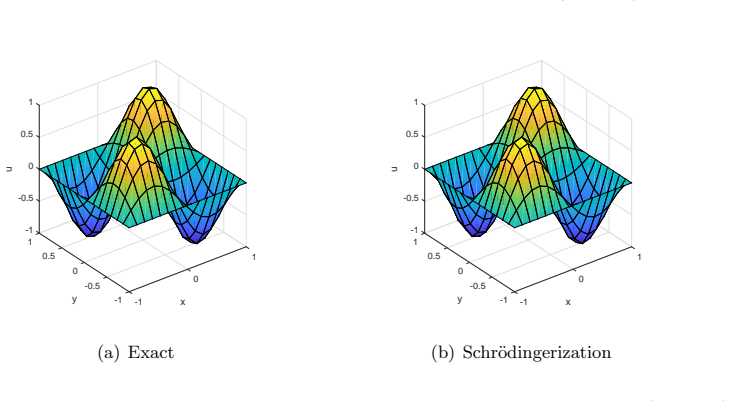
We develop a quantum algorithm for solving high-dimensional fractional Poisson equations. By applying the Caffarelli-Silvestre extension, the $d$-dimensional fractional equation is reformulated as a local partial differential equation in $d+1$ dimensions. We propose a quantum algorithm for the finite element discretization of this local problem, by capturing the steady-state of the corresponding differential equations using the Schr\"odingerization approach from \cite{JLY22SchrShort, JLY22SchrLong, analogPDE}. The Schr\"odingerization technique transforms general linear partial and ordinary differential equations into Schr\"odinger-type systems, making them suitable for quantum simulation. This is achieved through the warped phase transformation, which maps the equation into a higher-dimensional space. We provide detailed implementations of the method and conduct a comprehensive complexity analysis, which can show up to exponential advantage -- with respect to the inverse of the mesh size in high dimensions -- compared to its classical counterpart. Specifically, while the classical method requires $\widetilde{\mathcal{O}}(d^{1/2} 3^{3d/2} h^{-d-2})$ operations, the quantum counterpart requires $\widetilde{\mathcal{O}}(d 3^{3d/2} h^{-2.5})$ queries to the block-encoding input models, with the quantum complexity being independent of the dimension $d$ in terms of the inverse mesh size $h^{-1}$. Numerical experiments are conducted to verify the validity of our formulation.
Figures


Figures from the paper (5 more)


Forward citations
Cited by 1 Pith paper
-
A polynomial dimension-dependence analysis of Bramble--Pasciak--Xu preconditioners
Under convex-mesh assumptions, BPX preconditioner condition numbers for P1 finite elements grow at most polynomially in spatial dimension d, with explicit constants.
Reference graph
Works this paper leans on
-
[36]
S. Jin, N. Liu, C. Ma, and Y. Yu. On the Schr¨ odingerization method for linear non-unitary dynamics with optimal dependence on matrix queries. arXiv:2505.00370, 2025. 22
arXiv 2025
-
[25]
J. Hu, S. Jin, and L. Zhang. Quantum algorithms for multiscale partial differential equations. Multiscale Model. Simulation, 22:1030–1067, 2024
work page 2024
- [1]
-
[2]
G. Acosta and J. P. Borthagaray. A fractional Laplace equation: regularity of solutions and finite element approximations. SIAM J. Numer. Anal. , 55(2):472–495, 2015
work page 2015
-
[3]
G. Acosta and J. P. Borthagaray. A fractional Laplace equation: regularity of solutions and finite element approximations. SIAM J. Numer. Anal. , 55:472–495, 2017
work page 2017
-
[4]
D. An, A. M. Childs, and L. Lin. Quantum algorithm for linear non-unitary dynamics with near-optimal dependence on all parameters. arXiv:2312.03916, 2023
arXiv 2023
-
[5]
D. W. Berry. High-order quantum algorithm for solving linear differential equations. J. Phys. A: Math. Theor. , 47(10):105301, 17 pp., 2014
work page 2014
-
[6]
L. Caffarelli and L. Silvestre. An extension problem related to the fractional Laplacian. Com- mun. Part. Diff. Equ. , 32(8):1245–1260, 2007. 20
work page 2007
Show all 51 references
-
[7]
Y. Cao, S. Jin, and N. Liu. Quantum simulation for time-dependent Hamiltonians – with applications to non-autonomous ordinary and partial differential equations. arXiv:2312.02817, 2023
2023 arXiv
-
[8]
Y. Cao, S. Jin, and N. Liu. A unifying framework for quantum simulation algorithms for time-dependent Hamiltonian dynamics. arXiv:2411.03180, 2024
2024 arXiv
-
[9]
Y. Cao, A. Papageorgiou, I. Petras, et al. Quantum algorithm and circuit design solving the Poisson equation. New J. Phys. , 15:013021, 2013
2013
-
[10]
Carreras, V
B. Carreras, V. Lynch, and G. Zaslavsky. Anomalous diffusion and exit time distribution of particle tracers in plasma turbulence model. Phys. Plasmas., 8(12):5096–5103, 2001
2001
-
[11]
Chakraborty, A
S. Chakraborty, A. Gily´ en, and S. Jeffery. The power of block-encoded matrix powers: im- proved regression techniques via faster Hamiltonian simulation. In 46th International Col- loquium on Automata, Languages, and Programming (ICALP 2019) , volume 132 of Leibniz Internatio...
2019
-
[12]
A. M. Childs, R. Kothari, and R. D. Somma. Quantum algorithm for systems of linear equa- tions with exponentially improved dependence on precision. SIAM J. Comput. , 46(6):1920– 1950, 2017
1920
-
[13]
A. M. Childs, J. P. Liu, and A. Ostrander. High-precision quantum algorithms for partial differential equations. Quantum, 5:574, 2021
2021
-
[14]
A. W. Childs and J. Liu. Quantum spectral methods for differential equations. Comm. Math. Phys., 375(2):1427–1457, 2020
2020
-
[15]
P. C. S. Costa, S. Jordan, and A. Ostrander. Quantum algorithm for simulating the wave equation. Phys. Rev. A , 99:012323, 22 pp., 2019
2019
-
[16]
Q. Du. Nonlocal Modeling, Analysis, and Computationwings. Society for Industrial and Applied Mathematics, Philadelphia, PA, 2019
2019
-
[17]
Engel, G
A. Engel, G. Smith, and S. E. Parker. Quantum algorithm for the Vlasov equation. Phys. Rev. A, 100:062315, Dec 2019
2019
-
[18]
Gatto and J
P. Gatto and J. Hesthaven. Numerical approximation of the fractional Laplacian via hp-finite elements, with an application to image denoising. J. Sci. Comput. , 65:249–270, 2014
2014
-
[19]
Gily´ en, Y
A. Gily´ en, Y. Su, G. Low, and N. Wiebe. Quantum singular value transformation and beyond: exponential improvements for quantum matrix arithmetics. In Proceedings of the 51st Annual ACM SIGACT Symposium on Theory of Computing , pages 193–204. STOC, 2019
2019
-
[20]
Golse, S
F. Golse, S. Jin, and N. Liu. Quantum algorithms for uncertainty quantification: application to partial differential equations. arXiv:2209.11220, 2022. 21
2022 arXiv
-
[21]
Gu and M
Y. Gu and M. K. Ng. Deep ritz method for the spectral fractional Laplacian equation using the Caffarelli-Silvestre extension. SIAM J. Sci. Comput. , 44(4):A2018–A2036, 2022
2022
-
[22]
Z. Hao, Z. Cai, and Z. Zhang. Fractional-order dependent radial basis functions meshless methods for the integral fractional Laplacian. Comput. Math. Appl. , 178:197–213, 2025
2025
-
[23]
Hao and Z
Z. Hao and Z. Zhang. Optimal regularity and error estimates of a spectral Galerkin method for fractional advection-diffusion-reaction equations. SIAM J. Numer. Anal. , 58:211–233, 2020
2020
-
[24]
Z. Hao, Z. Zhang, and R. Du. Fractional centered difference scheme for high-dimensional integral fractional Laplacian. J. Comput. Phys. , 424:109851, 2021
2021
-
[26]
S. Jin, X. Li, N. Liu, and Y. Yu. Quantum simulation for partial differential equations with physical boundary or interface conditions. J. Comp. Phys. , 498:112707, 2024
2024
-
[27]
S. Jin, X. Li, N. Liu, and Y. Yu. Quantum simulation for quantum dynamics with artificial boundary conditions. SIAM J. Sci. Comput. , 46(4):B403–B421, 2024
2024
-
[28]
Jin and N
S. Jin and N. Liu. Analog quantum simulation of parabolic partial differential equations using Jaynes-Cummings-like models. arXiv:2407.01913, 2024
2024 arXiv
-
[29]
Jin and N
S. Jin and N. Liu. Analog quantum simulation of partial differential equations. Quantum Sci. Technol., 9(3):035047, 2024
2024
-
[30]
Jin and N
S. Jin and N. Liu. Quantum algorithms for nonlinear partial differential equations. Bull. Sci. math, 194:103457, 2024
2024
-
[31]
Jin and N
S. Jin and N. Liu. Quantum simulation of discrete linear dynamical systems and sim- ple iterative methods in linear algebra via Schr¨ odingerisation. Proc. Royal Soc. London A , 480(20230370), 2024
2024
-
[32]
S. Jin, N. Liu, and Ma. C. Quantum simulation of Maxwell’s equations via Schr¨ odingersation. Math. Model. Numer. Anal. , 58(5):1853–1879, 2024
2024
-
[33]
S. Jin, N. Liu, and C. Ma. On Schr¨ odingerization based quantum algorithms for linear dy- namical systems with inhomogeneous terms. arXiv:2402.14696, 2024
2024 arXiv
-
[34]
S. Jin, N. Liu, and C. Ma. Quantum circuits for the heat equation with physical boundary conditions via Schr¨ odingerisation.arXiv:2407.15895, 2024
2024 arXiv
-
[35]
S. Jin, N. Liu, and C. Ma. Schr¨ odingerisation based computationally stable algorithms for ill-posed problems in partial differential equations. arXiv:2403.19123, 2024
2024 arXiv
-
[37]
S. Jin, N. Liu, and W. Wei. Quantum algorithms for stochastic differential equations: A Schr¨ odingerisation approach.arXiv:2412.14868, 2024
2024 arXiv
-
[38]
S. Jin, N. Liu, and Y. Yu. Time complexity analysis of quantum difference methods for linear high dimensional and multiscale partial differential equations. J. Comput. Phys. , 471:111641, 2022
2022
-
[39]
S. Jin, N. Liu, and Y. Yu. Quantum simulation of partial differential equations: Applications and detailed analysis. Phys. Rev. A , 108:032603, 2023
2023
-
[40]
S. Jin, N. Liu, and Y. Yu. Quantum simulation of partial differential equations via Schr¨ odingerization.Phys. Rev. Lett., 133(23):230602, 2024
2024
-
[41]
S. Jin, N. Liu, and Y. Yu. Quantum simulation of the Fokker-Planck equation via Schr¨ odingerization.arXiv:2404.13585, 2024
2024 arXiv
-
[42]
Klafter and I
J. Klafter and I. Sokolov. Anomalous diffusion spreads its wings. Phys. World., 18:29, 2005
2005
-
[43]
L. Lin. Lecture notes on quantum algorithms for scientific computation. arXiv:2201.08309, 2022
2022 arXiv
-
[44]
Linden, A
N. Linden, A. Montanaro, and C. Shao. Quantum vs. classical algorithms for solving the heat equation. arXiv:2004.06516, 2020
2004 arXiv
-
[45]
C. Ma, S. Jin, N. Liu, K. Wang, and L. Zhang. Schr¨ odingerization based quantum circuits for Maxwell’s equation with time-dependent source terms. arXiv:2411.10999, 2024
2024 arXiv
-
[46]
Montanaro and S
A. Montanaro and S. Pallister. Quantum algorithms and the finite element method. Phys. Rev. A, 93:032324, 14 pp., 2016
2016
-
[47]
R. H. Nochetto, E. Ot´ arola, and A. J. Salgado. A PDE approach to fractional diffusion in general domains: A priori error analysis. Found Comput. Math., 15:733–791, 2015
2015
-
[48]
Sheng, B
C. Sheng, B. Su, and C. Xu. Efficient Monte Carlo method for integral fractional Laplacian in multiple dimensions. SIAM J. Numer. Anal. , 61:2035–2061, 2023
2023
-
[49]
J. L. V´ azquez. Recent progress in the theory of nonlinear diffusion with fractional Laplacian operators. Discrete Contin. Dyn. Syst. Ser. S , 7:857–885, 2014
2014
-
[50]
H. Yang, H. Chen, X. Yue, and G. Long. High-order fractional central difference method for multi-dimensional integral fractional Laplacian and its applications. Commun. Nonlinear Sci. Numer. Simul., 443:127757, 2023
2023
-
[51]
Y. Yang, J. Huang, Y. Wang, T. Deng, and H. Li. Fast Q1 finite element for two-dimensional integral fractional Laplacian. Appl. Math. Comput. , 443:127757, 2023. 23
2023
Reviewed August 16, 2026 · model on record in the stance chip above.
Discussion (0). Continue with ORCID to comment.