REVIEW 4 major objections 5 minor 58 references
Attractor-Based Coevolving Dot Product Random Graph Model
T0 review · 4 major / 5 minor · reviewed 2026-08-16 · deepseek-v4-flash
Pith's one-line read This paper introduces a dynamic random graph model in which each node's latent position moves toward same-group and cross-group attractors, and proves the influence parameters can be consistently estimated.
desk verdict The model is a genuinely useful RDPG-based dynamic latent space model, but the paper overclaims what is proven: the oracle-aligned consistency transfer (Theorem 7) has an internal gap, and no-oracle consistency is explicitly deferred to future work. read the letter →
The pith
A machine-rendered reading of the paper's core claim, the machinery that carries it, and where it could break.
The reading
What carries the argument
The load-bearing object is the attractor pair: $A^w_{i,t}$ is the average latent position of node $i$'s neighbors who share its group, and $A^b_{i,t}$ is the average over neighbors in other groups, with both averages taken over realized edges. Plugging these into a Dirichlet GLM creates the design matrix $X_t=[Z_t, A^w_t, A^b_t, \mathbf{1}_n]$, and the dynamics become $\alpha_{i,t+1}=\exp(X_{i,t}^T B)$, so inference on the social forces reduces to estimating $B$ and then projecting onto $\beta$. The argument succeeds because the attractor averages decorrelate asymptotically: conditioning on the latent positions, each row of the design matrix behaves like an independent row, so classical GLM consistency conditions (divergence, continuity, eigenvalue-ratio boundedness) apply. Latent positions are recovered by adjacency spectral embedding, and the paper handles the orthogonal non-identifiability of the random dot product graph with an oracle alignment in the theory and out-of-simplex penalty methods (SAE and GAEP) in practice.
What would settle it
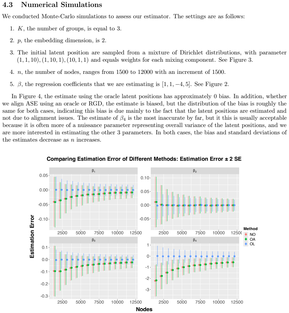
Run the Section 4.3 simulation at $n=12{,}000$ with the same $\beta=[1,1,-4,5]$ but alter the degree distribution so a positive fraction of nodes has expected within-group degree $D^*_i<\sqrt{\sigma}\,n$ for $\sigma\in\omega(n^{-1/2})\cap o(1)$; if the MLE of $\beta_3$ stays unbiased and the empirical-to-theoretical standard deviation ratio still approaches 1, the sparsity condition is not necessary for the claim as stated, whereas persistent bias or ratio drift would show the condition is doing the work.
Extended reading notes
Core claim
The central claim is that the dynamics have a tractable regression form: each node evolves as a Dirichlet generalized linear model with log link, $Z^*_{i,t+1} \sim \mathrm{Dir}(\exp(X_{i,t}^T B))$, where the design row $X_{i,t}$ stacks the node's current latent position, the within-group attractor $A^w_{i,t}$, the between-group attractor $A^b_{i,t}$, and a constant, and $B$ is a $(3p+1)\times(p+1)$ matrix that is a known linear function of the four influence coefficients $\beta$. Theorem 5 states that, under conditions controlling the expected within-group degree and the density of low-degree nodes, the MLE $\hat\beta$ asymptotically exists, is strongly consistent, and is asymptotically normal when the true latent positions are used. Theorem 7 and Corollary 2 extend this to observed networks: if the adjacency spectral embedding is aligned to the true latent positions by an oracle rotation, the plugin MLE still converges to the true parameter, with alignment error $O(\log^2(n)/\sqrt{n})$. The real-data analysis of competitive-game match networks finds a negative $\beta_3$ for a deliberately constructed 'away' group and a positive $\beta_3$ for a 'toward' group, matching the intended polarization and flocking.
Load-bearing premise
The load-bearing premise is that almost every node has enough same-group neighbors---expected within-group degree at least on the order of $\sqrt{\sigma}\,n$ with $\sigma$ tending to zero slower than $n^{-1/2}$---so that the attractor averages behave like independent rows and the design matrix is full rank; in sparse or highly polarized networks with many low-degree nodes this premise fails, and the paper's own no-oracle alignment consistency is also left as future work.
Editorial extensions
If this is right
- With two snapshots of a network, an analyst can estimate the four influence coefficients; the sign of $\beta_3$ indicates whether cross-group contact is attracting (flocking) or repelling (polarization).
- When the latent positions are known, the MLE of $\beta$ is consistent and asymptotically normal, so standard confidence intervals and hypothesis tests on the forces become available.
- Using oracle-aligned adjacency spectral embeddings, consistency of the plugin estimator is preserved, so the method scales to large networks because spectral embedding only requires a partial SVD.
- Because the model can be re-fit on each pair of consecutive snapshots, abrupt changes in $\beta$ over time are detectable from a longer time series.
- In the Age of Empires IV match network, the fitting procedure estimates $\beta_3<0$ for a group expected to polarize and $\beta_3>0$ for a group expected to flock, and the estimates are stable across embedding dimensions 3 through 9.
Reading between the lines
- If the theory extends to no-oracle alignment, polarization could be tested as a one-sided hypothesis on $\beta_3$, giving a principled alternative to modularity-based polarization indices; the paper explicitly leaves this no-oracle consistency proof to future work.
- A practical pitfall follows from the oracle assumption: if the two time points are aligned to different rotations, the estimated $\beta$ will be biased in a way that does not vanish with $n$. A testable extension is to compare SAE/GAEP-aligned estimates with oracle-aligned estimates across $n$ and check whether the gap shrinks at the promised rate.
- The attractor definition assumes hard group labels and a fixed node set, so applying the model to opinion spectra or to networks with nodes arriving and leaving would require mixed-membership and node-varying extensions, both named by the paper as future directions.
Signed reviews
Editorial analysis
A structured set of objections, weighed in public.
Referee Report
Summary. The manuscript proposes the Attractor-Based Coevolving Dot Product Random Graph Model (ABCDPRGM), a temporal RDPG model in which latent positions evolve according to a Dirichlet GLM whose predictors are the current latent position and within- and between-group neighbor attractors. Estimation is two-stage: latent positions are recovered by adjacency spectral embedding (ASE), and the coefficients β are then estimated by Dirichlet GLM maximum likelihood. The theoretical results are Theorem 5 (asymptotic existence, consistency, and asymptotic normality when latent positions are known), Theorem 7 (stability of the MLE under 2→∞-consistent latent-position estimates), and Corollary 2 (consistency when ASE is aligned to the true latent positions by an oracle). The paper also reports simulations and an analysis of Age of Empires IV match data aimed at detecting polarization and flocking.
Significance. The model is a natural and analytically attractive dynamic extension of RDPG, and the known-latent-position part of the proof follows a recognizable Fahrmeir-Kaufmann GLM framework with explicit Bernstein-type bounds. If the transfer theorems are correct, the framework provides a tractable way to quantify polarizing and flocking forces from two network snapshots. The simulations are informative and the real-data analysis is useful as an illustration. However, the practical claim of consistency with estimated latent positions is currently proved only under an oracle alignment, the proof of Theorem 7 has an internal assumption mismatch, and the real-data inference uses standard errors that ignore latent-position estimation uncertainty. These issues are fixable, but they materially affect the paper's central claims.
major comments (4)
- [Section 4.2, Theorem 7] The proof of Theorem 7 uses an assumption that is not stated in the theorem. The theorem's assumption 2 only requires max_{i≤n,j≤p+1} exp{X_{i*}^T B_{*j}} > 2, but the proof asserts 'By assumption, α_ij > 2+C0 for some fixed C0 in R+' and then applies Lemma 9, which requires the first parameter a of each Beta distribution to exceed 2 for E[Z^{-2}] to be finite. The max condition does not imply a uniform lower bound on all α_ij. For example, with p=1, β1=-10, β2=β3=0, β4=1, a node with Z_i1 near 1 has α_i1 = exp(-10 Z_i1 + 1) < 2 while α_i2 = exp(-10 Z_i2 + 1) > 2, so max > 2 holds but some components have α_ij ≤ 2; for those components E[Z_ij^{-2}] is infinite and the Chebyshev bound in the proof fails. Since the bound ||\tilde{B} - \hat{B}||_2 = O_p(ε) is the entire content of the theorem, the ASE-to-MLE consistency transfer is not established as stated. Replacing the assumption by min_{i,j} α_ij > 2+C0, or some other uniform lower bound, would repair the proof, but that condition then needs to be stated and checked in applications.
- [Section 4.2, Corollary 2, and Section 6] The consistency result for observed networks is limited to an oracle alignment. Corollary 2 states that there exists W_s ∈ O_p such that \hat{Z}_s W_s is consistent for Z_s, but it does not provide a data-driven construction of W_s. Section 6 explicitly defers proofs for the no-oracle methods to future work. The real-data analysis in Section 5 uses GAEP, which has no consistency theorem, so the estimator used in the application is not covered by Corollary 2. The abstract and Section 3.1 should be reworded to state clearly that consistency is proved for oracle-aligned ASE plus known latent positions, while the no-oracle alignment methods are supported only by simulations.
- [Section 5, Table 4 and Figure 5] The reported 'theoretical standard deviations' are the Fisher-information standard errors from the Dirichlet GLM evaluated at the estimated latent positions, and they do not account for uncertainty in ASE, alignment, or dimension selection. The text uses these standard errors to suggest that the null β3 = 0 would be rejected for the away group. This inference is not justified as stated, because the variance of the two-stage estimator is at least as large as the GLM variance conditional on estimated positions. A variance estimator that accounts for latent-position estimation, or an explicit statement that this is an informal diagnostic, is needed before the real-data evidence can support the claimed polarization detection.
- [Section 5.1 and 5.2] The real-data validation is weakened by the way the groups are constructed. The away group is defined as players whose MMR trend is consistent with polarization (low-skilled players who got worse versus high-skilled players who got better), and the same MMR-trend variable is then used to interpret β3 as evidence of polarization. This makes the empirical 'detection' partly built into the group construction. The paper should acknowledge this selection issue and provide an additional analysis that does not use the outcome variable to define the groups, for example using a holdout period or pre-registered group definitions based only on period-0 information.
minor comments (5)
- [Appendix A.1] The proof of Theorem 5 begins with 'We first prove Theorem 2', but the theorem being proved is Theorem 5; the cross-reference is incorrect.
- [Section 4.3 / Figure 5] The caption of Figure 5 says the color code is identical to that of 'Figure 4.3'; it should refer to Figure 4.
- [Section 3.3] The text introduces GAEP and SAE but the simulations refer to a method labeled 'RGD'; the relationship between RGD, SAE, and GAEP should be stated explicitly so that it is clear which estimator is used in each simulation and in the real-data analysis.
- [Throughout] There are numerous typographical and wording errors, including 'qauntifies', 'convinience', 'unecessary', 'nuissance', 'polariation', and 'mispecified'. A careful proofreading pass is needed.
- [Section 4.1] The assumption in Theorem 5 that the normalized degree density satisfies f(x) ≤ k_b x^{-δ_b} with δ_b < 1 and σ ∈ ω(n^{-1/2}) is substantive; the paper should state clearly that the asymptotic theory applies to relatively dense network regimes and does not cover very sparse or heavily polarized networks where many nodes have low expected degree.
Circularity Check
No significant circularity: the estimation theory is a self-contained likelihood derivation, and the real-data group construction is a selected validation sample rather than an algebraic reduction of the estimated parameter to its inputs.
full rationale
The paper's central derivation is not circular. The ABCDPRGM defines latent-position evolution through a Dirichlet GLM with design matrix X_t = [Z_t, A^w_t, A^b_t, 1_n] and parameter matrix B (Eq. 2). The MLE is obtained by maximizing the likelihood ℓ(B|Z*) and its consistency/asymptotic normality are derived from standard GLM conditions (D), (N), (S) in the proof of Theorem 5. The key difficulty, dependence among rows of X through the attractors, is handled by replacing X with an asymptotically independent approximation bX and proving ||X_Λg - bX_Λg||_{2→∞} = o_p(1) via Lemmas 1-5. Nothing in this chain defines B in terms of the estimator or fits a parameter and then renames it a prediction. Theorem 7 transfers consistency to oracle-aligned ASE estimates via the implicit function theorem and bounds on score-function derivatives (Lemmas 8-9); this is a genuine analytic argument, not a self-citation chain. The citation to [2] for ASE consistency is external published theory (even though one author overlaps) and does not assume the target result. The real-data analysis does construct the 'away' and 'toward' groups using MMR trends that are expected to exhibit polarization or flocking, and Table 4 reports β3 = -0.4141 for the away group with a negative sign consistent with that expectation. This is a selected validation sample, but β3 is not defined in terms of MMR trend; it is estimated from the latent-position transition model. There is no equation in the paper making the estimated β3 equal to the group-construction outcome by construction. A separate correctness concern, not a circularity, is that the proof of Theorem 7 asserts 'By assumption, α_ij > 2 + C0' and applies Lemma 9, which needs the Beta first parameter a > 2 for every component, whereas Assumption 2 of Theorem 7 only states max_{i,j} exp{X_i*^T B_*j} > 2. This is an internal theorem/proof gap about a uniform lower bound, not a reduction of the conclusion to its inputs. Accordingly, the circularity score is 0.
Assumptions & free parameters
free parameters (7)
- beta_1 (self-influence) =
1.5946 (real data; simulated truth 1)
- beta_2 (within-group attractor) =
1.6428 (real data; simulated truth 1)
- beta_3 (between-group attractor) =
-0.4141 (real data; simulated truth -4)
- beta_4 (nuisance) =
1.1258 (real data; simulated truth 5)
- embedding dimension p =
5 for real data, checked over 2 to 9
- GAEP penalty lambda and softplus temperature mu
- alignment rotations W_0, W_1 =
not reported
assumptions (9)
- domain assumption RDPG edge distribution: conditioning on Z_t, entries of Y_t are independent Bernoulli with P(Y_ij,t=1)=Z_i,t^T Z_j,t.
- domain assumption At t=0, latent positions Z_i,0 are i.i.d. Dirichlet with parameters drawn i.i.d. from F supported on the simplex.
- domain assumption Latent positions evolve as Z_i,t+1 ~ Dir(exp{X_i,t B}), a Dirichlet GLM with log link.
- domain assumption Node set and group membership labels are fixed and known.
- domain assumption Expected degree density near zero is bounded as f(x) <= k_b x^{-delta_b} with delta_b<1, and most nodes satisfy D_i^* >= sqrt(sigma)n.
- domain assumption The expected Fisher information from the independent-rows approximation is positive definite.
- ad hoc to paper There exist orthogonal matrices W_s such that bZ_s W_s is a consistent estimate of Z_s.
- ad hoc to paper For the proof of Theorem 7, each Dirichlet concentration parameter satisfies alpha_ij > 2 + C0.
- standard math Existing GLM asymptotic theory (Fahrmeir and Kaufmann) and ASE consistency (Athreya et al.) apply as cited.
invented entities (1)
-
within-group and between-group attractors A_w, A_b
Cite this review
Pith. "Pith review of Attractor-Based Coevolving Dot Product Random Graph Model." pith.science (2026). https://pith.science/paper/E6LHW6M6
@misc{pith2026250502675,
  author       = {Pith},
  title        = {Pith review of: Attractor-Based Coevolving Dot Product Random Graph Model},
  year         = {2026},
  howpublished = {\url{https://pith.science/paper/E6LHW6M6}},
  note         = {Machine review of arXiv:2505.02675}
}
read the original abstract
We introduce the attractor-based coevolving dot product random graph model (ABCDPRGM) to analyze time-series network data manifesting polarizing or flocking behavior. Graphs are generated based on latent positions under the random dot product graph regime. We assign group membership to each node. When evolving through time, the latent position of each node will change based on its current position and two attractors, which are defined to be the centers of the latent positions of all of its neighbors who share its group membership or who have different group membership than it. Parameters are assigned to the attractors to quantify the amount of influence that the attractors have on the trajectory of the latent position of each node. We developed estimators for the parameters, demonstrated their consistency, and established convergence rates under specific assumptions. Through the ABCDPRGM, we provided a novel framework for quantifying and understanding the underlying forces influencing the polarizing or flocking behaviors in dynamic network data.
Figures


Figures from the paper (7 more)


Reference graph
Works this paper leans on
-
[1]
Lada A. Adamic and Natalie Glance. The political blogosphere and the 2004 u.s. election: divided they blog. In Proceedings of the 3rd International Workshop on Link Discovery, LinkKDD ’05, page 36–43, New York, NY, USA, 2005. Association for Computing Machinery
work page 2004
-
[2]
Avanti Athreya, Donniell E. Fishkind, Minh Tang, Carey E. Priebe, Youngser Park, Joshua T. Vogelstein, Keith Levin, Vince Lyzinski, Yichen Qin, and Daniel L Sussman. Statistical inference on random dot product graphs: a survey.Journal of Machine Learning Research, 18(226):1–92, 2018
work page 2018
-
[3]
Sur les opérations dans les ensembles abstraits et leur application aux équations intégrales
Stefan Banach. Sur les opérations dans les ensembles abstraits et leur application aux équations intégrales. Fundamenta Mathematicae, 3:133–181, 1922
1922
-
[4]
Bishop.Pattern Recognition and Machine Learning
Christopher M. Bishop.Pattern Recognition and Machine Learning. Springer, 2006
2006
-
[5]
An Introduction to Optimization on Smooth Manifolds
Nicolas Boumal. An Introduction to Optimization on Smooth Manifolds. Cambridge University Press, 2023
2023
-
[6]
George Casella and Roger L. Berger.Statistical Inference. Duxbury, 2nd edition, 2002
work page 2002
-
[7]
Michael Conover, Jacob Ratkiewicz, Matthew Francisco, Bruno Goncalves, Filippo Menczer, and Alessandro Flammini. Political polarization on twitter.Proceedings of the International AAAI Conference on Web and Social Media, 5(1):89–96, 8 2021
work page 2021
-
[8]
Ludwig Fahrmeir and Heinz Kaufmann. Consistency and asymptotic normality of the maximum likelihood estimator in generalized linear models.The Annals of Statistics, 13(1):342 – 368, 1985
work page 1985
Show all 58 references
-
[9]
Gradient- based spectral embeddings of random dot product graphs.arXiv preprint arXiv:2307.13818, 2023
Marcelo Fiori, Bernardo Marenco, Federico Larroca, Paola Bermolen, and Gonzalo Mateos. Gradient- based spectral embeddings of random dot product graphs.arXiv preprint arXiv:2307.13818, 2023. Machine Learning (cs.LG); Optimization and Control (math.OC)
2023 arXiv
-
[10]
On the properties of the softmax function with application in game theory and reinforcement learning.arXiv preprint arXiv:1704.00805, 2017
Bolin Gao and Lacra Pavel. On the properties of the softmax function with application in game theory and reinforcement learning.arXiv preprint arXiv:1704.00805, 2017. 17
2017 arXiv
-
[11]
A measure of polarization on social media networks based on community boundaries.Proceedings of the International AAAI Conference on Web and Social Media, 7(1):215–224, 8 2021
Pedro Guerra, Wagner Meira Jr., Claire Cardie, and Robert Kleinberg. A measure of polarization on social media networks based on community boundaries.Proceedings of the International AAAI Conference on Web and Social Media, 7(1):215–224, 8 2021
2021
-
[12]
Dynamic hidden-variable network models
Harrison Hartle, Fragkiskos Papadopoulos, and Dmitri Krioukov. Dynamic hidden-variable network models. Physical Review E, 103(5):052307, 2021
2021
-
[13]
Mixed membership estimation for social networks
Jiashun Jin, Zheng Tracy Ke, and Shengming Luo. Mixed membership estimation for social networks. Journal of Econometrics, 239(2):105369, 2024
2024
-
[14]
Longford
Nicholas T. Longford. A fast scoring algorithm for maximum likelihood estimation in unbalanced mixed models with nested random effects.Biometrika, 74(4):817–827, 1987
1987
-
[15]
William Marthy and Damien R. Farine. The potential impacts of the songbird trade on mixed-species flocking. Biological Conservation, 222:222–231, 2018
2018
-
[16]
Coordinate descent on the orthogonal group for recurrent neural network training
Estelle Massart and Vinayak Abrol. Coordinate descent on the orthogonal group for recurrent neural network training. Proceedings of the AAAI Conference on Artificial Intelligence, 36(7):7744–7751, 6 2022
2022
-
[17]
McCright and Riley E
Aaron M. McCright and Riley E. Dunlap. The politicization of climate change and polarization in the american public’s views of global warming, 2001–2010.The Sociological Quarterly, 52(2):155–194, 2011
2001
-
[18]
Nelder.Generalized Linear Models
Peter McCullagh and John A. Nelder.Generalized Linear Models. Monographs on Statistics and Applied Probability. Chapman and Hall, 2nd edition, 1989
1989
-
[19]
Munkres.Analysis on Manifolds
James R. Munkres.Analysis on Manifolds. CRC Press, 1st edition, 1991
1991
-
[20]
A model for the co-evolution of dynamic social networks and infectious disease dynamics.Computational Social Networks, 8(1):19, 2021
Hendrik Nunner, Vincent Buskens, and Mirjam Kretzschmar. A model for the co-evolution of dynamic social networks and infectious disease dynamics.Computational Social Networks, 8(1):19, 2021
2021
-
[21]
Olesen, Constantí Stefanescu, and Anna Traveset
Jens M. Olesen, Constantí Stefanescu, and Anna Traveset. Strong, long-term temporal dynamics of an ecological network.PLOS ONE, 6(11):1–5, 11 2011
2011
-
[22]
Dynamic stochastic blockmodel regression for network data
Santiago Olivella, Tyler Pratt, and Kosuke Imai. Dynamic stochastic blockmodel regression for network data. Journal of the American Statistical Association, 117(538):929–942, 2022
2022
-
[23]
Christenson, Konstantinos Spiliopoulos, Dylan Walker, and Eric D
Hancong Pan, Xiaojing Zhu, Cantay Caliskan, Dino P. Christenson, Konstantinos Spiliopoulos, Dylan Walker, and Eric D. Kolaczyk. Stochastic gradient descent-based inference for dynamic network models with attractors. arXiv preprint arXiv:2403.07124, 2024
2024 arXiv
-
[24]
Latent space approaches to social network analysis
Adrian E Raftery Peter D Hoff and Mark S Handcock. Latent space approaches to social network analysis. Journal of the American Statistical Association, 97(460):1090–1098, 2002
2002
-
[25]
Dynamic social network analysis using latent space models
Purnamrita Sarkar and Andrew Moore. Dynamic social network analysis using latent space models. In Y. Weiss, B. Schölkopf, and J. Platt, editors,Advances in Neural Information Processing Systems, volume 18. MIT Press, 2005
2005
-
[26]
Sewell and Yuguo Chen
Daniel K. Sewell and Yuguo Chen. Latent space models for dynamic networks.Journal of the American Statistical Association, 110(512):1646–1657, 2015
2015
-
[27]
Sewell and Yuguo Chen
Daniel K. Sewell and Yuguo Chen. Latent space models for dynamic networks.Journal of the American Statistical Association, 110(512):1646–1657, October 2015
2015
-
[28]
Foundations and modeling of dynamic networks using dynamic graph neural networks: A survey.IEEE Access, 9:79143–79168, 2021
Joakim Skarding, Bogdan Gabrys, and Katarzyna Musial. Foundations and modeling of dynamic networks using dynamic graph neural networks: A survey.IEEE Access, 9:79143–79168, 2021
2021
-
[29]
A review of latent space models for social networks, 2020
Juan Sosa and Lina Buitrago. A review of latent space models for social networks, 2020. 18
2020
-
[30]
Cambridge University Press, 2018
Roman Vershynin.High-Dimensional Probability: An Introduction with Applications in Data Science, volume 47 ofCambridge Series in Statistical and Probabilistic Mathematics. Cambridge University Press, 2018
2018
-
[31]
Xu and Alfred O
Kevin S. Xu and Alfred O. Hero III. Dynamic stochastic blockmodels: Statistical models for time-evolving networks. IEEE Journal of Selected Topics in Signal Processing, 8(4):552–562, 2014
2014
-
[32]
Zavlanos, Ali Jadbabaie, and George J
Michael M. Zavlanos, Ali Jadbabaie, and George J. Pappas. Flocking while preserving network connec- tivity. In2007 46th IEEE Conference on Decision and Control, pages 2919–2924, 12 2007
2007
-
[33]
Xiaojing Zhu, Cantay Caliskan, Dino P Christenson, Konstantinos Spiliopoulos, Dylan Walker, and Eric D Kolaczyk. Disentangling positive and negative partisanship in social media interactions using a coevolving latent space network with attractors model.Journal of the Royal Sta...
2023
-
[34]
Z is in Rn×(p+1) such that its row sum vector is a constant1 vector
-
[35]
X is the design matrix fromZt
-
[36]
Z will exclusively refer toZt+1
-
[37]
any decorated version ofX,Z are defined analogously 21
-
[38]
We shall first invoke the implicit function theorem (IFT)[19]
Any matrix with a subscriptv is its vectorized version, e.g.Bv = Vec(B),Xv = Vec(X), etc. We shall first invoke the implicit function theorem (IFT)[19]. In short, this theorem tells us that there is a unique continuously differentiable function,g, that maps data to MLE. Theref...
-
[39]
There is an open setU⊂ Rn×q× Rn×(p+1) containing (X,Z ), whereq = 3p + 1
-
[40]
There is a unique continuously differentiable functiong : U → Rq(p+1) that satisfies the following conditions: (a) g(X,Z ) = bBv, (b) ∀(X∗,Z∗)∈U, ∂ ∂Bv [ℓ (B∗ v;X∗,Z∗)] = 0, whereB∗ v =g(X∗,Z∗). In addition,∀(X∗,Z∗)∈U, ∂g (R,S) ∂(R,S) (R,S)=(X ∗,Z∗) is characterized in the fol...
-
[41]
bBv =g(X,Z ), this is the true MLE from the true latent positions,(X,Z )
-
[42]
realistic
˜Bv =g ˜X, ˜Z , this is the “realistic” MLE from the estimated latent postions, ˜X, ˜Z
-
[43]
Now we proceed to show that the MLE,˜B, computed using the approximations,˜X, ˜Z gets sufficiently close to the true MLE,bB with n large enough
B∗ v =g (X∗,Z∗), this is some MLE from some arbitary latent positions(X∗,Z∗) near (X,Z ). Now we proceed to show that the MLE,˜B, computed using the approximations,˜X, ˜Z gets sufficiently close to the true MLE,bB with n large enough. Define Λ(ϵ) ={i∈V|Zi∗∈Dp(ϵ)} to be the set...
-
[44]
estimate
that lead to4. Lemma 1. For allλ> 0: P (∥Ni−N∗ i∥2≥λn)≤ 2p exp −2λ2n p P (|Di−D∗ i|≥ λn)≤ 2 exp −2λ2n Proof. P 1 n∥Ni−N∗ i∥2≥λ ≤P 1 n∥Ni−N∗ i∥∞≥ λ√p = E P 1 n∥Ni−N∗ i∥∞≥ λ√p Z = E P 1 n X j∈τ(i) YijZj− X j∈τ(i) E(Yij)Zj ∞ ≥ λ√p Z = E P p[ l=1 1 n X ...
-
[45]
Lemma 6 guarantees that after deleting data, we still have enough left for inference, and Lemma 8, 9 helps us characterize the functiong
So we need to shave off the portion of our data that is near 0. Lemma 6 guarantees that after deleting data, we still have enough left for inference, and Lemma 8, 9 helps us characterize the functiong. Lemma 7 is about showing that under our assumptions, ASE is consistent, whi...
-
[46]
Pn i=1 1 {Zi,0∈A} = ΘP (n),
-
[47]
Pn i=1 1 {Zi,t∈A} = ΘP (n) =⇒ Pn i=1 1 {Zi,t+1∈A} = ΘP (n). Proof. Att = 0, by assumptionZi,0 are non-degenerate i.i.d. Dirichlet random variables fori = 1,...,n . Let µ be the Lebesgue measure forRp. For allA⊂ ∆p with µ(A)> 0,∃δ >0 such that∀x∈A, fZi,0(x)>δ . Therefore P (Zi,...
-
[48]
λp ZtZT t = Θp(n), whereλp(A) = the pth largest singular value ofA,
-
[49]
If the above conditions holds, then forbZt, the ASE-estimate ofZt: min W∈Op Zt− bZtW 2→∞ ≤ C log2(n) δ1/2 ZtZT t
δ ZtZT t = Θp(n), whereδ(P ) = maxi P jPij. If the above conditions holds, then forbZt, the ASE-estimate ofZt: min W∈Op Zt− bZtW 2→∞ ≤ C log2(n) δ1/2 ZtZT t . 29 Proof. First we prove thatλp ZtZT t = Θp(n): Let b1,...,b p be a basis of∆p. LetAk be an open neighborhood ofbk for...
2000
-
[50]
The response variables,{yi}n i=1 are independent random variables within the same exponential family but have different natural parameters{θi}n i=1,
-
[51]
Explanatory variablesZi∈ Rp influences yi in form of a linear combination,γi =ZT i β, whereβ is the parameter of the GLM with appropriate dimensions,
-
[52]
32 D.1.2 Conditions for Consistency and Asymptotic Normality In this section, we shall assumeβ0 to be the true parameter
γi is related toµ(θi) = E [t(yi)] by some injective link functiong, more specifically,γi = (g◦µ)(θi). 32 D.1.2 Conditions for Consistency and Asymptotic Normality In this section, we shall assumeβ0 to be the true parameter. For notational convenience, theβ0 argument in any fun...
-
[53]
Initialize at someW∈Op
-
[54]
Compute the Euclidean gradient atW, Le(W ) = ∂ ∂W [L(W )]
-
[55]
Compute the Riemannian gradient atW that is given by the orthogonal projection ofLe(W ) to the tangent space ofOp at W,TWOp: (a) TWOp = WA A∈ Rp×p and AT =−A , (b) The orthogonal projection is given by PTWOp(M) =W WTM−MTW 2 , (4) (c) The Riemannian gradient atW: Lr(W ) =PTWOp(Le(W ))
-
[56]
Take a gradient descent step in the tangent space using the Riemannian gradient: W tangent t+1 =Wt−αLr(Wt), where α is some appropriate step size
-
[57]
This retraction is done through the matrix exponential function, Expm: Wt+1 =WtExpm WT t W tangent t+1
Retract the result from previous step back toOp. This retraction is done through the matrix exponential function, Expm: Wt+1 =WtExpm WT t W tangent t+1
-
[58]
Iterate step 2 to step 5 until convergence. 34
Reviewed August 16, 2026 · model on record in the stance chip above.
Discussion (0). Continue with ORCID to comment.