REVIEW 2 major objections 6 minor 131 references
The Absolute Age of Milky Way Globular Clusters
T0 review · 2 major / 6 minor · reviewed 2026-08-16 · deepseek-v4-flash
Pith's one-line read This paper derives absolute ages for eight Milky Way globular clusters—11.5 to 13.5 Gyr—by fitting Monte Carlo isochrone ensembles to space-based photometry, and reports a clear trend of older age at lower metallicity.
desk verdict Careful absolute-age pipeline for eight GCs; the 2D-KS assumption for five clusters needs testing before the 0.5–0.75 Gyr errors are taken at face value. read the letter →
The pith
A machine-rendered reading of the paper's core claim, the machinery that carries it, and where it could break.
The reading
What carries the argument
The central machinery is a Monte Carlo isochrone ensemble: for each of the eight clusters, 10,000 draws from 21 stellar-evolution parameters produce isochrone sets from 8 to 16 Gyr, and each isochrone is expanded into a synthetic color-magnitude diagram of 4 million stars using the cluster's mass function, binary fraction, and artificial-star-test photometric errors. Fitting compares the observed and synthetic cumulative distributions via the 2D Kolmogorov–Smirnov statistic, calibrated by a bootstrap empirical null distribution, or via Voronoi-binned $\chi^2$ density comparisons for the crowded clusters. A calibration-star $\chi^2$ weight is multiplied into the CMD-fit weight, and Johnson indices decompose the age variance into per-parameter contributions. This machinery is what lets the paper report absolute ages with an explicit error budget rather than relative rankings.
What would settle it
Re-analyze M55 (or NGC 4147) with artificial star tests that include exposure-to-exposure PSF variations; if the best-fit age moves by more than about 0.5 Gyr or synthetic recovery tests show the 2D KS fit is biased when PSF scatter is underestimated, the quoted 0.5-0.75 Gyr uncertainties for the sparse clusters are too small.
Extended reading notes
Core claim
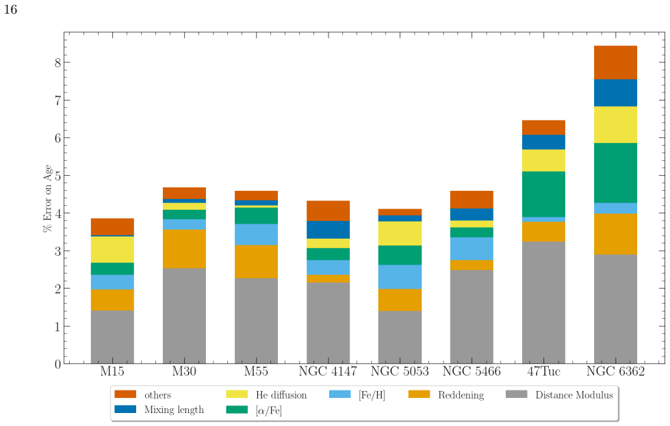
At the heart of the paper is a Monte Carlo ensemble of stellar evolution models: for each cluster, 10,000 draws from 21 physics parameters (nuclear reaction rates, opacities, convective mixing, diffusion, boundary conditions, and more) yield isochrone sets spanning 8–16 Gyr. Each isochrone is converted into a synthetic color-magnitude diagram of 4 million stars that includes the cluster's mass function, binary fraction, and photometric scatter and completeness from artificial star tests. The observed CMD is then fit with two full-CMD methods—Voronoi binning for the crowded clusters M15, M30, and 47 Tuc, and a 2D Kolmogorov-Smirnov ECDF comparison for the sparser clusters—with bootstrap resampling defining the null distribution that assigns each isochrone its weight; calibration stars with precise parallaxes and, where available, detached eclipsing binaries provide independent checks. The claim is that the resulting absolute ages run from $11.61 \pm 0.98$ Gyr for NGC 6362 to $13.23 \pm 0.51$ Gyr for M15, that distance and reddening account for over half the age uncertainty, and that the combined sample yields the first absolute age-metallicity relation for Milky Way globular clusters, with older ages at lower metallicity.
Load-bearing premise
For the five less crowded clusters (M55, NGC 4147, NGC 5053, NGC 5466, NGC 6362), the 2D Kolmogorov-Smirnov statistic is assumed to remain an unbiased age estimator even though the artificial-star tests underestimate photometric scatter from PSF modeling; the paper states this uncertainty cannot be quantified without redesigning the artificial-star test process.
Editorial extensions
If this is right
- All eight clusters fall within about $1\sigma$ of the cosmic microwave background age of the universe, so globular clusters remain viable as independent lower bounds on cosmic age.
- The discovered age-metallicity trend implies the most metal-poor clusters formed earliest, and the paper proposes extending the analysis to metal-rich clusters to map the full relation.
- Since distance and reddening contribute over half the age uncertainty, better distances (for example from eclipsing binaries or improved parallaxes) would directly shrink age errors without changing the stellar models.
- Multiple stellar populations do not disturb the age estimate: the two 47 Tuc subpopulations fit to the same age within uncertainties, so single-population models are adequate for the filters used.
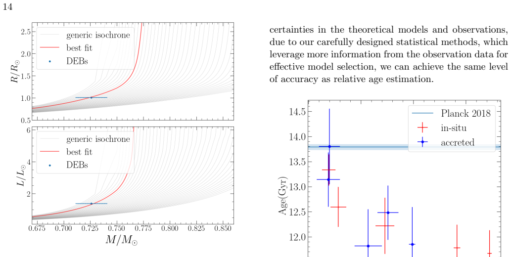
- Independent detached-eclipsing-binary fits for 47 Tuc and NGC 6362 give ages consistent with the CMD fits, cross-validating the method on different data.
Reading between the lines
- If distance really dominates the error budget, applying the same pipeline to clusters with detached-eclipsing-binary distances should cut age errors by roughly the square root of that share; the paper's own DEB age for 47 Tuc ($11.36 \pm 0.81$ Gyr) is already competitive, suggesting this is testable now.
- The 2D KS method's claimed robustness to PSF scatter could be validated by injecting synthetic photometric errors with known PSF mismatch into a simulated CMD; if recovered ages stay unbiased, the five sparse-cluster ages rest on firmer ground.
- The absolute age-metallicity relation, if extended toward $[\mathrm{Fe/H}] \approx -0.5$, could discriminate between in-situ disk formation and accretion scenarios, since the in-situ sequence is predicted to turn over at low metallicity.
- Because the oldest and most metal-poor clusters sit near 13 Gyr, a plausible reading is that metal-poor globular cluster formation began within about a billion years of the Big Bang, tightening the timeline for early Milky Way assembly; the paper itself does not claim this explicitly.
Signed reviews
Editorial analysis
A structured set of objections, weighed in public.
Referee Report
Summary. The paper determines absolute ages for eight Milky Way globular clusters by fitting HST ACS F606W/F814W color-magnitude diagrams with Monte Carlo isochrones from the Dartmouth Stellar Evolution Program. The isochrones sample 21 stellar evolution parameters, and the fitting uses synthetic CMDs with artificial-star-test photometric errors, a calibration-star prior on the stellar physics, and two full-CMD statistics: a Voronoi binning chi-square method for the crowded clusters M15, M30, and 47 Tuc, and a 2D Kolmogorov-Smirnov method for M55, NGC 4147, NGC 5053, NGC 5466, and NGC 6362. The paper reports ages of 11.5-13.5 Gyr with typical 0.5-0.75 Gyr uncertainties, finds distance and reddening to be the dominant error sources, and presents an age-metallicity relation for ten clusters when combined with earlier work.
Significance. If the results hold, this would be a valuable step toward absolute globular cluster ages with a quantified stellar-physics error budget, and the age-metallicity trend shown in Figure 11 would be an interesting constraint on early Milky Way assembly. The paper has real strengths: the Monte Carlo isochrone catalog is released on Zenodo, the pipeline is described in enough detail to be reproduced, the two fitting methods agree well for the three clusters where both are applied, and the detached-eclipsing-binary checks for 47 Tuc and NGC 6362 provide an independent consistency test. The main weakness is the unquantified PSF-related photometric scatter for the five less crowded clusters, whose ages come solely from the 2D KS method without a validation that the method is unbiased under this systematic mismatch.
major comments (2)
- [Sec. 4.1, 4.2; Figs. 2, 3; Table 7] The ages of M55, NGC 4147, NGC 5053, NGC 5466, and NGC 6362 are derived exclusively from the 2D KS method, yet the paper states in Section 4.1 that for these clusters the artificial star tests underestimate photometric scatter because the PSF model cannot match the true PSF, and that 'it is impossible to quantify the uncertainty due to the PSF modeling without redesigning the AS test process'. Section 4.2 asserts that the cumulative nature of the 2D KS statistic attenuates this width mismatch, but no synthetic test or analytic argument is provided to show that the 2D KS age estimator remains unbiased under this mismatch. Since the missing PSF scatter can depend on stellar brightness and local crowding, the ECDF distortion is likely age-dependent: as the trial age moves the turn-off to different magnitudes, the effect of the width mismatch on the KS statistic changes. In addition, the bootstrap null distribution constructed in Section 4.2 (step 2) uses the same underestimated scatter, so both the central ages and the quoted 0.5-0.75 Gyr uncertainties for these five clusters omit an unquantified systematic. This directly affects the age-metallicity relation in Figure 11, which leans heavily on these five clusters. I request a quantitative robustness test, for example injecting an extra magnitude-dependent scatter comparable to the observed width mismatch into synthetic CMDs and checking that the input ages are recovered within the stated uncertainties, or an explicit systematic error term added to the affected ages.
- [Table 2; Sec. 5.1, Eq. (5)] Table 2 lists no calibration star for NGC 5053 or NGC 5466, yet Section 5.1 and Equation (5) combine a calibration weight w_Cali with the CMD weight for every cluster. If these two clusters lack suitable field-star calibrators, the absolute zero point of their ages is not anchored by the calibration-star procedure, and it is unclear what value of w_Cali was used. If they are intended to share calibrators from other clusters, the [Fe/H] and [alpha/Fe] matching should be stated explicitly. This is load-bearing for the absolute age scale of two of the eight clusters and needs to be clarified or corrected in the text and table.
minor comments (6)
- [Table 2] The table lists only one star per cluster row while the text says M55 uses two calibration stars, HD103269 and HD108200; please make explicit which calibration stars are used for each cluster, since the current table layout is ambiguous and appears to use the same stars for M55 and NGC 4147.
- [Sec. 5.1, Fig. 11] The claim to present the 'first absolute age-metallicity relation for Milky Way GCs' is too strong as stated, given that earlier works such as VandenBerg et al. (2013), which is cited in Table 7, provide absolute ages for many clusters; please either qualify the novelty (for example, as the first relation based on a full Monte Carlo stellar-parameter error budget) or soften the wording.
- [Sec. 4.2] The description of the Gaussian-process optimization of distance and reddening is brief; please specify the kernel, the number of iterations, the convergence criterion, and how the boundary values from Table 4 are enforced, so that the procedure is fully reproducible.
- [Sec. 4.2] The bootstrap null distribution is built from the single best-fitting base model selected using the same data; this selection can make the null distribution too narrow. A short discussion or test of this effect would strengthen the weight assignment.
- [Sec. 4.1, Eq. (2)] In the chi-square metric, please clarify whether E_i is normalized to the total observed star count and how bins with zero expected counts are treated, since these choices affect the fitted weights.
- [Table 5] The present-day mass function and binary fraction are fixed to literature values without propagated uncertainties; the paper should state why these choices do not materially affect the turn-off age determination, or include them in the error budget.
Circularity Check
No significant circularity: absolute ages are anchored by independent calibration stars and eclipsing binaries, and cross-checked against external literature ages.
full rationale
The paper's absolute ages are derived by fitting Monte Carlo isochrone sets to HST photometry, with stellar physics parameters sampled from literature-based distributions (Tables 1 and 4). The calibration-star weights (Section 5.1) come from field main-sequence stars with Gaia EDR3 parallaxes and HST photometry, not from cluster members, so they constrain model physics without encoding the cluster age. Detached eclipsing binaries (Table 3) are independent data (masses, luminosities, radii) from published light-curve analyses, not from the CMD fit. The 2D KS and Voronoi methods were developed in the authors' prior papers (Ying et al. 2023, 2024), but they are statistical tools applied to new cluster data rather than results assumed as input; the paper also compares against external literature ages (Table 7), and the DEB-based ages for 47 Tuc and NGC 6362 agree with the CMD-based ages. The admitted PSF scatter underestimation in the AS tests (Section 4.1) and the unvalidated robustness of the 2D KS method to that mismatch are validity and robustness concerns, not circularity: the paper does not define the age in terms of the fit statistic, and no fitted target result is reused as a 'prediction' by construction. No equation or fitted parameter in the derivation chain reduces to an assumed output, so no circular step can be exhibited.
Assumptions & free parameters
free parameters (25)
- Distance modulus mu, M15 (NGC 7078) =
15.45 +/- 0.03
- Reddening E(V-I), M15 (NGC 7078) =
0.08 +/- 0.01
- Distance modulus mu, M30 (NGC 7099) =
14.82 +/- 0.05
- Reddening E(V-I), M30 (NGC 7099) =
0.03 +/- 0.01
- Distance modulus mu, M55 (NGC 6809) =
14.03 +/- 0.05
- Reddening E(V-I), M55 (NGC 6809) =
0.10 +/- 0.01
- Distance modulus mu, NGC 4147 =
16.48 +/- 0.03
- Reddening E(V-I), NGC 4147 =
0.01 +/- 0.01
- Distance modulus mu, NGC 5053 =
16.25 +/- 0.04
- Reddening E(V-I), NGC 5053 =
0.01 +/- 0.01
- Distance modulus mu, NGC 5466 =
16.14 +/- 0.06
- Reddening E(V-I), NGC 5466 =
0.02 +/- 0.01
- Distance modulus mu, 47 Tuc (NGC 104) =
13.37 +/- 0.05
- Reddening E(V-I), 47 Tuc (NGC 104) =
0.02 +/- 0.01
- Distance modulus mu, NGC 6362 =
14.69 +/- 0.06
- Reddening E(V-I), NGC 6362 =
0.06 +/- 0.01
- [Fe/H] (sampled per cluster with Gaussian priors, marginalised) =
Posterior means: M15 -2.31, M30 -2.23, M55 -1.77, NGC4147 -1.74, NGC5053 -2.31, NGC5466 -1.93, 47Tuc -0.78, NGC6362…
- [alpha/Fe] (sampled per cluster, marginalised)
- Gaia EDR3 parallax zero-point correction factor (calibration stars) =
0.5 (half of Lindegren et al. 2021 correction)
- Mixing length parameter alpha_MLT =
uniform 1.0 to 2.5
- Convective core overshoot =
uniform 0 to 0.2
- Convective envelope overshoot =
uniform 0 to 0.2
- Helium diffusion coefficient scaling =
uniform 0.5 to 1.3
- Heavy element diffusion scaling =
uniform 0.5 to 1.3
- Delta Y / Delta Z enrichment ratio =
uniform 1.75 to 2.5
assumptions (6)
- domain assumption MC parameter ranges in Table 1 bracket the true physics of low-mass stellar evolution
- ad hoc to paper The calibrated isochrone luminosity scale is correctly anchored by the two field calibration stars and the Gaia EDR3 parallax zero-point treatment
- domain assumption The 2D KS statistic remains an unbiased age estimator despite the AS-test width mismatch for less crowded clusters
- domain assumption Multiple stellar populations do not significantly affect the F606W and F814W CMD morphology used for age fitting
- domain assumption The adopted PDMF and binary fraction in Table 5 describe the observed populations
- domain assumption DSEP stellar models and PHOENIX bolometric corrections are accurate representations of real stars
Cite this review
Pith. "Pith review of The Absolute Age of Milky Way Globular Clusters." pith.science (2026). https://pith.science/paper/NKJVFJU6
@misc{pith2026250502969,
  author       = {Pith},
  title        = {Pith review of: The Absolute Age of Milky Way Globular Clusters},
  year         = {2026},
  howpublished = {\url{https://pith.science/paper/NKJVFJU6}},
  note         = {Machine review of arXiv:2505.02969}
}
abstract
Globular clusters (GCs) provide statistically significant coeval populations of stars spanning various evolutionary stages, allowing robust constraints on stellar evolution model parameters and ages. We analyze eight old Milky Way GCs with metallicities between [Fe/H] $=-2.31$ and $-0.77$ by comparing theoretical isochrone sets from the Dartmouth Stellar Evolution Program to HST observations. The theoretical isochrones include uncertainties introduced by $21$ stellar evolution parameters such as convective mixing, opacity, diffusion, and nuclear reactions, capturing much of the quantifiable physics used in our code. For each isochrone, we construct synthetic color-magnitude diagrams (CMD) near the main-sequence turn-off region and apply two full-CMD-fitting methods to fit HST ACS data across a range of distance and reddening and measure the absolute age of each GC from the resulting posterior distribution, which accounts for uncertainties in the stellar models, observations, and fitting method. The resulting best-fitting absolute ages range from $\approx 11.5$ to $13.5$ Gyr, with a typical error of $0.5-0.75$ Gyr; the data show a clear trend toward older ages at lower metallicities. Notably, distance and reddening account for over $50\%$ of the uncertainty in age determination in each case, with metallicity, $\alpha$ abundance, mixing length, and helium diffusion being the most important stellar physics parameters for the error budget. We also provide an absolute age-metallicity relation for Milky Way GCs.
Figures


Figures from the paper (8 more)





Reference graph
Works this paper leans on
-
[1]
2016, Physics Letters B, 760, 584, doi: 10.1016/j.physletb.2016.07.032
Platter, L. 2016, Physics Letters B, 760, 584, doi: 10.1016/j.physletb.2016.07.032
-
[2]
Adamo, A., Bradley, L. D., Vanzella, E., et al. 2024, The Discovery of Bound Star Clusters 460 Myr after the Big Bang, doi: 10.48550/arXiv.2401.03224
-
[3]
G., Garc´ ıa, A., Robertson, R
Adelberger, E. G., Garc´ ıa, A., Robertson, R. G. H., et al. 2011, Reviews of Modern Physics, 83, 195, doi: 10.1103/RevModPhys.83.195 Alvarez Garay, D. A., Mucciarelli, A., Lardo, C., Bellazzini, M., & Merle, T. 2022, ApJL, 928, L11, doi: 10.3847/2041-8213/ac5ccf
-
[4]
2009, ApJL, 697, L58, doi: 10.1088/0004-637X/697/1/L58
Guhathakurta, P. 2009, ApJL, 697, L58, doi: 10.1088/0004-637X/697/1/L58
-
[5]
Anderson, J., Sarajedini, A., Bedin, L. R., et al. 2008, AJ, 135, 2055, doi: 10.1088/0004-6256/135/6/2055
-
[6]
Arnold, J. A., Romanowsky, A. J., Brodie, J. P., et al. 2011, ApJL, 736, L26, doi: 10.1088/2041-8205/736/2/L26
-
[7]
Aver, E., Olive, K. A., & Skillman, E. D. 2015, JCAP, 2015, 011, doi: 10.1088/1475-7516/2015/07/011
-
[8]
J., & Feigelson, E
Babu, G. J., & Feigelson, E. D. 2006, in Astronomical Data Analysis Software and Systems XV, Vol. 351, 127
2006
Show all 131 references
-
[9]
2021, MNRAS, 505, 5957, doi: 10.1093/mnras/stab1474
Baumgardt, H., & Vasiliev, E. 2021, MNRAS, 505, 5957, doi: 10.1093/mnras/stab1474
2021 doi
-
[10]
2024, MNRAS, 528, 3198, doi: 10.1093/mnras/stad3920
Belokurov, V., & Kravtsov, A. 2024, MNRAS, 528, 3198, doi: 10.1093/mnras/stad3920
2024 doi
-
[11]
Bentley, J. L. 1980, Communications of the ACM, 23, 214, doi: 10.1145/358841.358850
1980
-
[12]
2021, ApJ, 922, 20, doi: 10.3847/1538-4357/ac214d
Yang, S.-C. 2021, ApJ, 922, 20, doi: 10.3847/1538-4357/ac214d
2021 doi
-
[13]
1986, ˚ ap, 162, 21
Bica, E., & Alloin, D. 1986, ˚ ap, 162, 21
1986
-
[14]
M., Friel, E
Boberg, O. M., Friel, E. D., & Vesperini, E. 2015, ApJ, 804, 109, doi: 10.1088/0004-637X/804/2/109
2015 doi
-
[15]
D., Basu, S., et al
Bonaca, A., Tanner, J. D., Basu, S., et al. 2012, ApJL, 755, L12, doi: 10.1088/2041-8205/755/1/L12
2012 doi
-
[16]
2023, fidanka
Boudreaux, E., & Ying, M. 2023, fidanka. https://github.com/tboudreaux/fidanka
2023
-
[17]
M., Chaboyer, B
Boudreaux, E. M., Chaboyer, B. C., Ash, A., Edaes Hoh, R., & Feiden, G. 2025, ApJ, 980, 180, doi: 10.3847/1538-4357/ad9740
2025 doi
-
[18]
Boylan-Kolchin, M., & Weisz, D. R. 2021, MNRAS, 505, 2764, doi: 10.1093/mnras/stab1521
2021 doi
-
[19]
A., Bedin, L
Brogaard, K., VandenBerg, D. A., Bedin, L. R., et al. 2017, MNRAS, 468, 645, doi: 10.1093/mnras/stx378
2017 doi
-
[20]
1970, ApJ, 159, 641, doi: 10.1086/150338
Canuto, V. 1970, ApJ, 159, 641, doi: 10.1086/150338
1970 doi
-
[21]
2003, MNRAS, 342, 345, doi: 10.1046/j.1365-8711.2003.06541.x
Cappellari, M., & Copin, Y. 2003, MNRAS, 342, 345, doi: 10.1046/j.1365-8711.2003.06541.x
2003
-
[22]
2009a, ˚ ap, 508, 695, doi: 10.1051/0004-6361/200913003
Lucatello, S. 2009a, ˚ ap, 508, 695, doi: 10.1051/0004-6361/200913003
-
[23]
G., et al
Carretta, E., Bragaglia, A., Gratton, R. G., et al. 2009b, A&A, 505, 117, doi: 10.1051/0004-6361/200912096
-
[24]
2008, ApJL, 672, L115, doi: 10.1086/527035
Cassisi, S., Salaris, M., Pietrinferni, A., et al. 2008, ApJL, 672, L115, doi: 10.1086/527035
2008 doi
-
[25]
J., Krauss, L
Chaboyer, B., Demarque, P., Kernan, P. J., Krauss, L. M., & Sarajedini, A. 1996, MNRAS, 283, 683, doi: 10.1093/mnras/283.2.683
1996 doi
-
[26]
1995, ApJ, 454, 767, doi: 10.1086/176529
Chaboyer, B., & Kim, Y.-C. 1995, ApJ, 454, 767, doi: 10.1086/176529
1995 doi
-
[27]
E., O’Malley, E., et al
Chaboyer, B., McArthur, B. E., O’Malley, E., et al. 2017, ApJ, 835, 152, doi: 10.3847/1538-4357/835/2/152
2017 doi
-
[28]
2015, PhRvC, 91, 045801, doi: 10.1103/PhysRevC.91.045801
Chakraborty, S., deBoer, R., Mukherjee, A., & Roy, S. 2015, PhRvC, 91, 045801, doi: 10.1103/PhysRevC.91.045801
2015 doi
-
[29]
2016, ApJ, 823, 102, doi: 10.3847/0004-637X/823/2/102
Choi, J., Dotter, A., Conroy, C., et al. 2016, ApJ, 823, 102, doi: 10.3847/0004-637X/823/2/102
2016 doi
-
[30]
2020, ApJ, 900, 146, doi: 10.3847/1538-4357/aba829
Chun, S.-H., Lee, J.-J., & Lim, D. 2020, ApJ, 900, 146, doi: 10.3847/1538-4357/aba829
2020 doi
-
[31]
J., Pilachowski, C
Cordero, M. J., Pilachowski, C. A., Johnson, C. I., et al. 2014, ApJ, 780, 94, doi: 10.1088/0004-637X/780/1/94 deBoer, R. J., G¨ orres, J., Smith, K., et al. 2014, Phys. Rev. C, 90, 035804, doi: 10.1103/PhysRevC.90.035804 19
2014 doi
-
[32]
Ferguson, J. W. 2017, ApJ, 849, 159, doi: 10.3847/1538-4357/aa92c9
2017 doi
-
[33]
2016, ApJS, 222, 8, doi: 10.3847/0067-0049/222/1/8
Dotter, A. 2016, ApJS, 222, 8, doi: 10.3847/0067-0049/222/1/8
2016 doi
-
[34]
2008, ApJ Supplement Series, 178, 89, doi: 10.1086/589654
Dotter, A., Chaboyer, B., Jevremovi´ c, D., et al. 2008, ApJ Supplement Series, 178, 89, doi: 10.1086/589654
2008 doi
-
[35]
W., Conroy, C., et al
Dotter, A., Ferguson, J. W., Conroy, C., et al. 2015, MNRAS, 446, 1641, doi: 10.1093/mnras/stu2170
2015 doi
-
[36]
2010, ApJ, 708, 698, doi: 10.1088/0004-637X/708/1/698
Dotter, A., Sarajedini, A., Anderson, J., et al. 2010, ApJ, 708, 698, doi: 10.1088/0004-637X/708/1/698
2010 doi
-
[37]
1999, SIAM Review, 41, 637, doi: 10.1137/S0036144599352836
Du, Q., Faber, V., & Gunzburger, M. 1999, SIAM Review, 41, 637, doi: 10.1137/S0036144599352836
1999 doi
- [38]
-
[39]
2020, MNRAS, 494, 4226, doi: 10.1093/mnras/staa969
Hilker, M. 2020, MNRAS, 494, 4226, doi: 10.1093/mnras/staa969
2020 doi
-
[40]
Eddington, A. S. 1926, The Internal Constitution of the Stars (Cambridge University Press)
1926
-
[41]
2019, MNRAS, 482, 4528, doi: 10.1093/mnras/sty3007
Boylan-Kolchin, M. 2019, MNRAS, 482, 4528, doi: 10.1093/mnras/sty3007
2019 doi
-
[42]
1987, MNRAS, 225, 155, doi: 10.1093/mnras/225.1.155
Fasano, G., & Franceschini, A. 1987, MNRAS, 225, 155, doi: 10.1093/mnras/225.1.155
1987 doi
-
[43]
W., Alexander, D
Ferguson, J. W., Alexander, D. R., Allard, F., et al. 2005, ApJ, 623, 585, doi: 10.1086/428642
2005 doi
-
[44]
Ferguson, T. S. 1973, The Annals of Statistics, 1, 209 , doi: 10.1214/aos/1176342360
1973
-
[45]
K., Paust, N
Feuillet, D. K., Paust, N. E. Q., & Chaboyer, B. 2014, PASP, 126, 733, doi: 10.1086/677845 Gaia Collaboration, Brown, A. G. A., Vallenari, A., et al. 2021, ˚ ap, 649, A1, doi: 10.1051/0004-6361/202039657
2014 doi
-
[46]
2018, MNRAS, 475, L15, doi: 10.1093/mnrasl/slx203
Giesers, B., Dreizler, S., Husser, T.-O., et al. 2018, MNRAS, 475, L15, doi: 10.1093/mnrasl/slx203
2018 doi
-
[47]
2019, A&A, 632, A3, doi: 10.1051/0004-6361/201936203
Giesers, B., Kamann, S., Dreizler, S., et al. 2019, A&A, 632, A3, doi: 10.1051/0004-6361/201936203
2019 doi
-
[48]
A., Khovritchev, M
Gontcharov, G. A., Khovritchev, M. Y., Mosenkov, A. V., et al. 2023a, MNRAS, 518, 3036, doi: 10.1093/mnras/stac3300
-
[49]
A., Bonatto, C
Gontcharov, G. A., Bonatto, C. J., Ryutina, O. S., et al. 2023b, MNRAS, 526, 5628, doi: 10.1093/mnras/stad3134
-
[50]
A., Savchenko, S
Gontcharov, G. A., Savchenko, S. S., Marchuk, A. A., et al. 2024, Research in Astronomy and Astrophysics, 24, 065014, doi: 10.1088/1674-4527/ad420f H¨ aberle, M., Neumayer, N., Seth, A., et al. 2024, Nature, 631, 285, doi: 10.1038/s41586-024-07511-z
2024 doi
-
[51]
1994, ApJ, 425, 222, doi: 10.1086/173978
Haft, M., Raffelt, G., & Weiss, A. 1994, ApJ, 425, 222, doi: 10.1086/173978
1994 doi
-
[52]
Harris, W. E. 1996, AJ, 112, 1487, doi: 10.1086/118116
1996 doi
-
[53]
H., Allard, F., & Baron, E
Hauschildt, P. H., Allard, F., & Baron, E. 1999, ApJ, 512, 377, doi: 10.1086/306745
1999 doi
-
[54]
2019, ApJS, 243, 7, doi: 10.3847/1538-4365/ab1f72
Huang, Y., Chen, B.-Q., Yuan, H.-B., et al. 2019, ApJS, 243, 7, doi: 10.3847/1538-4365/ab1f72
2019 doi
-
[55]
B., & Lampe, M
Hubbard, W. B., & Lampe, M. 1969, ApJ Supplement Series, 18, 297, doi: 10.1086/190192
1969 doi
-
[56]
O., Wende-von Berg, S., Dreizler, S., et al
Husser, T. O., Wende-von Berg, S., Dreizler, S., et al. 2013, ˚ ap, 553, A6, doi: 10.1051/0004-6361/201219058
2013 doi
-
[57]
1983, ARA&A, 21, 271, doi: 10.1146/annurev.aa.21.090183.001415
Iben, Jr., I., & Renzini, A. 1983, ARA&A, 21, 271, doi: 10.1146/annurev.aa.21.090183.001415
1983
- [58]
-
[59]
Irwin, A. W. 2012, Astrophysics Source Code Library, ascl:1211.002
2012
-
[60]
1998, Proceedings of the National Academy of Sciences, 95, 13, doi: 10.1073/pnas.95.1.13
Jimenez, R. 1998, Proceedings of the National Academy of Sciences, 95, 13, doi: 10.1073/pnas.95.1.13
1998 doi
-
[61]
1996, ApJ, 463, L17, doi: 10.1086/310053
Jimenez, R., & Padoan, P. 1996, ApJ, 463, L17, doi: 10.1086/310053
1996 doi
-
[62]
Johnson, J. W. 2000, Multivariate Behavioral Research, 35, 1, doi: 10.1207/S15327906MBR3501 1
2000 doi
-
[63]
2018, ApJ, 856, 10, doi: 10.3847/1538-4357/aab200
Joyce, M., & Chaboyer, B. 2018, ApJ, 856, 10, doi: 10.3847/1538-4357/aab200
2018 doi
-
[64]
2023, Galaxies, 11, 75, doi: 10.3390/galaxies11030075
Joyce, M., & Tayar, J. 2023, Galaxies, 11, 75, doi: 10.3390/galaxies11030075
2023 doi
-
[65]
M., Arellano Ferro, A., et al
Kains, N., Bramich, D. M., Arellano Ferro, A., et al. 2013, A&A, 555, A36, doi: 10.1051/0004-6361/201321819
2013 doi
- [66]
-
[67]
B., Krzeminski, W., et al
Kaluzny, J., Thompson, I. B., Krzeminski, W., et al. 2005, in Stellar Astrophysics with the World’s Largest
2005
-
[68]
N., Guhathakurta, P., & Sneden, C
Kirby, E. N., Guhathakurta, P., & Sneden, C. 2008, ApJ, 682, 1217, doi: 10.1086/589627
2008 doi
-
[69]
2008, AJ, 135, 1551, doi: 10.1088/0004-6256/135/4/1551 Kov´ acs, G., & Walker, A
Koch, A., & McWilliam, A. 2008, AJ, 135, 1551, doi: 10.1088/0004-6256/135/4/1551 Kov´ acs, G., & Walker, A. R. 2001, A&A, 371, 579, doi: 10.1051/0004-6361:20010346
2008 doi
-
[70]
M., & Chaboyer, B
Krauss, L. M., & Chaboyer, B. 2003, Science, 299, 65, doi: 10.1126/science.1075631 Krishna Swamy, K. S. 1966, ApJ, 145, 174, doi: 10.1086/148752
2003 doi
-
[71]
L., Babusiaux, C., & Cox, N
Lallement, R., Vergely, J. L., Babusiaux, C., & Cox, N. L. J. 2022, A&A, 661, A147, doi: 10.1051/0004-6361/202142846
2022 doi
-
[72]
P., Venn, K
Lamb, M. P., Venn, K. A., Shetrone, M. D., Sakari, C. M., & Pritzl, B. J. 2015, MNRAS, 448, 42, doi: 10.1093/mnras/stu2674
2015 doi
-
[73]
2022, A&A, 662, A117, doi: 10.1051/0004-6361/202243843 20
Lardo, C., Salaris, M., Cassisi, S., & Bastian, N. 2022, A&A, 662, A117, doi: 10.1051/0004-6361/202243843 20
2022 doi
-
[74]
S., Beers, T
Lee, Y. S., Beers, T. C., Allende Prieto, C., et al. 2011, AJ, 141, 90, doi: 10.1088/0004-6256/141/3/90
2011 doi
-
[75]
V., Milone, A
Legnardi, M. V., Milone, A. P., Cordoni, G., et al. 2023, MNRAS, 522, 367, doi: 10.1093/mnras/stad1056
2023 doi
-
[76]
2021, ˚ ap, 649, A4, doi: 10.1051/0004-6361/202039653
Lindegren, L., Bastian, U., Biermann, M., et al. 2021, ˚ ap, 649, A4, doi: 10.1051/0004-6361/202039653
2021 doi
-
[77]
H., Merenda, P
Lindeman, R. H., Merenda, P. F., & Gold, R. Z. 1980, Introduction to Bivariate and Multivariate Analysis (Glenview, Ill.: Scott, Foresman)
1980
-
[78]
E., Schiavilla, R., & Viviani, M
Marcucci, L. E., Schiavilla, R., & Viviani, M. 2013, PhRvL, 110, 192503, doi: 10.1103/PhysRevLett.110.192503 Mar´ ın-Franch, A., Aparicio, A., Piotto, G., et al. 2009, ApJ, 694, 1498, doi: 10.1088/0004-637X/694/2/1498
2013 doi
-
[79]
F., Milone, A
Marino, A. F., Milone, A. P., Dondoglio, E., et al. 2023, ApJ, 958, 31, doi: 10.3847/1538-4357/acfca3
2023 doi
-
[80]
2011, PhRvC, 83, 045804, doi: 10.1103/PhysRevC.83.045804
Marta, M., Formicola, A., Bemmerer, D., et al. 2011, PhRvC, 83, 045804, doi: 10.1103/PhysRevC.83.045804
2011 doi
-
[81]
2017, MNRAS, 468, 1249, doi: 10.1093/mnras/stx549
Massari, D., Mucciarelli, A., Dalessandro, E., et al. 2017, MNRAS, 468, 1249, doi: 10.1093/mnras/stx549
2017 doi
-
[82]
P., & Marino, A
Milone, A. P., & Marino, A. F. 2022, Universe, 8, 359, doi: 10.3390/universe8070359
2022 doi
-
[83]
P., Piotto, G., Bedin, L
Milone, A. P., Piotto, G., Bedin, L. R., et al. 2012, A&A, 540, A16, doi: 10.1051/0004-6361/201016384
2012 doi
-
[84]
P., Marino, A
Milone, A. P., Marino, A. F., Renzini, A., et al. 2018, MNRAS, 481, 5098, doi: 10.1093/mnras/sty2573
2018 doi
- [85]
-
[86]
G., Desprez, G., et al
Mowla, L., Iyer, K. G., Desprez, G., et al. 2022, ApJL, 937, L35, doi: 10.3847/2041-8213/ac90ca
2022 doi
-
[87]
2016, ApJ, 824, 73, doi: 10.3847/0004-637X/824/2/73
Mucciarelli, A., Dalessandro, E., Massari, D., et al. 2016, ApJ, 824, 73, doi: 10.3847/0004-637X/824/2/73
2016 doi
-
[88]
B., et al
Olech, A., Kaluzny, J., Thompson, I. B., et al. 2001, MNRAS, 321, 421, doi: 10.1046/j.1365-8711.2001.04010.x O’Malley, E. M., Gilligan, C., & Chaboyer, B. 2017a, ApJ, 838, 162, doi: 10.3847/1538-4357/aa6574 O’Malley, E. M., McWilliam, A., Chaboyer, B., &
2001
-
[89]
2017b, ApJ, 838, 90, doi: 10.3847/1538-4357/aa62a2
Thompson, I. 2017b, ApJ, 838, 90, doi: 10.3847/1538-4357/aa62a2
-
[90]
Paust, N. E. Q., Chaboyer, B., & Sarajedini, A. 2007, AJ, 133, 2787, doi: 10.1086/513511
2007 doi
-
[91]
Paust, N. E. Q., Reid, I. N., Piotto, G., et al. 2010, AJ, 139, 476, doi: 10.1088/0004-6256/139/2/476
2010 doi
-
[92]
Peacock, J. A. 1983, MNRAS, 202, 615, doi: 10.1093/mnras/202.3.615
1983 doi
- [93]
- [94]
-
[95]
1990, ApJ, 350, 662, doi: 10.1086/168418
Djorgovski, S. 1990, ApJ, 350, 662, doi: 10.1086/168418
1990 doi
-
[96]
R., Anderson, J., et al
Piotto, G., Bedin, L. R., Anderson, J., et al. 2007, ApJL, 661, L53, doi: 10.1086/518503 Planck Collaboration, Aghanim, N., Akrami, Y., et al. 2020, A&A, 641, A6, doi: 10.1051/0004-6361/201833910
2007 doi
- [97]
-
[98]
2019, MNRAS, 483, 1674, doi: 10.1093/mnras/sty3208
Valenzuela-Calderon, C. 2019, MNRAS, 483, 1674, doi: 10.1093/mnras/sty3208
2019 doi
- [99]
-
[100]
G., Casertano, S., Yuan, W., et al
Riess, A. G., Casertano, S., Yuan, W., et al. 2021, ApJL, 908, L6, doi: 10.3847/2041-8213/abdbaf
2021 doi
-
[101]
Rodriguez, C. L. 2023, ApJ, 947, L12, doi: 10.3847/2041-8213/acc9b6
2023 doi
-
[102]
Rousseeuw, P. J. 1987, Journal of Computational and Applied Mathematics, 20, 53, doi: https://doi.org/10.1016/0377-0427(87)90125-7
1987 doi
- [103]
-
[104]
L., Bolte, M., Langer, G
Sandquist, E. L., Bolte, M., Langer, G. E., Hesser, J. E., & de Oliveira, C. M. 1999, ApJ, 518, 262, doi: 10.1086/307268
1999 doi
-
[105]
2011, The ACS Survey of Galactic Globular Clusters (”ACSGGCT”), STScI/MAST, doi: 10.17909/T9TG65
Sarajedini, A. 2011, The ACS Survey of Galactic Globular Clusters (”ACSGGCT”), STScI/MAST, doi: 10.17909/T9TG65. http://archive.stsci.edu/doi/ resolve/resolve.html?doi=10.17909/T9TG65
2011 doi
-
[106]
1990, ApJ, 365, 219, doi: 10.1086/169472
Sarajedini, A., & Demarque, P. 1990, ApJ, 365, 219, doi: 10.1086/169472
1990 doi
-
[107]
R., Chaboyer, B., et al
Sarajedini, A., Bedin, L. R., Chaboyer, B., et al. 2007, AJ, 133, 1658, doi: 10.1086/511979
2007 doi
-
[108]
2015, A&A, 579, A104, doi: 10.1051/0004-6361/201425509
Sbordone, L., Monaco, L., Moni Bidin, C., et al. 2015, A&A, 579, A104, doi: 10.1051/0004-6361/201425509
2015 doi
-
[109]
F., & Finkbeiner, D
Schlafly, E. F., & Finkbeiner, D. P. 2011, ApJ, 737, 103, doi: 10.1088/0004-637X/737/2/103
2011 doi
-
[110]
R., & Nicholas, C
Shahapure, K. R., & Nicholas, C. 2020, in 2020 IEEE 7th International Conference on Data Science and Advanced Analytics (DSAA), 747–748
2020
-
[111]
H., Miller, B., et al
Simunovic, M., Puzia, T. H., Miller, B., et al. 2023, ApJ, 950, 135, doi: 10.3847/1538-4357/acce3d
2023 doi
-
[112]
2017, MNRAS, 471, 3668, doi: 10.1093/mnras/stx1856
Sollima, A., & Baumgardt, H. 2017, MNRAS, 471, 3668, doi: 10.1093/mnras/stx1856
2017 doi
-
[113]
B., Vandenberg, D
Stetson, P. B., Vandenberg, D. A., & Bolte, M. 1996, PASP, 108, 560, doi: 10.1086/133766 21
1996 doi
-
[114]
G., Geisler, D., et al
Tang, B., Fern´ andez-Trincado, J. G., Geisler, D., et al. 2018, ApJ, 855, 38, doi: 10.3847/1538-4357/aaaaea
2018 doi
-
[115]
D., Basu, S., & Demarque, P
Tanner, J. D., Basu, S., & Demarque, P. 2014, ApJL, 785, L13, doi: 10.1088/2041-8205/785/1/L13
2014 doi
-
[116]
B., Udalski, A., Dotter, A., et al
Thompson, I. B., Udalski, A., Dotter, A., et al. 2020, MNRAS, 492, 4254, doi: 10.1093/mnras/staa032
2020 doi
-
[117]
A., Bahcall, J
Thoul, A. A., Bahcall, J. N., & Loeb, A. 1994, ApJ, 421, 828, doi: 10.1086/173695
1994 doi
-
[118]
2013, ApJ, 775, 134, doi: 10.1088/0004-637X/775/2/134
Casagrande, L. 2013, ApJ, 775, 134, doi: 10.1088/0004-637X/775/2/134
2013 doi
-
[119]
A., & Denissenkov, P
VandenBerg, D. A., & Denissenkov, P. A. 2018, ApJ, 862, 72, doi: 10.3847/1538-4357/aaca9b
2018 doi
-
[120]
A., Denissenkov, P
VandenBerg, D. A., Denissenkov, P. A., & Catelan, M. 2016, ApJ, 827, 2, doi: 10.3847/0004-637X/827/1/2
2016 doi
-
[121]
Ferguson, J. W. 2022, MNRAS, 509, 4189, doi: 10.1093/mnras/stab2996
2022 doi
-
[122]
2021, MNRAS, 505, 5978, doi: 10.1093/mnras/stab1475
Vasiliev, E., & Baumgardt, H. 2021, MNRAS, 505, 5978, doi: 10.1093/mnras/stab1475
2021 doi
-
[123]
2016, MNRAS, 460, 2351, doi: 10.1093/mnras/stw1146
Villanova, S., Monaco, L., Moni Bidin, C., & Assmann, P. 2016, MNRAS, 460, 2351, doi: 10.1093/mnras/stw1146
2016 doi
-
[124]
M., Villante, F
Vinyoles, N., Serenelli, A. M., Villante, F. L., et al. 2017, ApJ, 835, 202, doi: 10.3847/1538-4357/835/2/202
2017 doi
-
[125]
2023, MNRAS, 522, 5740, doi: 10.1093/mnras/stad1068
Vitral, E., Libralato, M., Kremer, K., et al. 2023, MNRAS, 522, 5740, doi: 10.1093/mnras/stad1068
2023 doi
-
[126]
2017, A&A, 607, A135, doi: 10.1051/0004-6361/201730976
Wang, Y., Primas, F., Charbonnel, C., et al. 2017, A&A, 607, A135, doi: 10.1051/0004-6361/201730976
2017 doi
-
[127]
2013, Nuclear Physics A, 918, 61, doi: 10.1016/j.nuclphysa.2013.09.007
Xu, Y., Takahashi, K., Goriely, S., et al. 2013, Nuclear Physics A, 918, 61, doi: 10.1016/j.nuclphysa.2013.09.007
2013 doi
-
[128]
M., Chaboyer, B., Boudreaux, E
Ying, J. M., Chaboyer, B., Boudreaux, E. M., et al. 2023, AJ, 166, 18, doi: 10.3847/1538-3881/acd9b1
2023 doi
-
[129]
M., Chaboyer, B., & Du, W
Ying, J. M., Chaboyer, B., & Du, W. 2024, ApJ, 970, 184, doi: 10.3847/1538-4357/ad59a9
2024 doi
-
[130]
S., & Norris, J
Yong, D., Da Costa, G. S., & Norris, J. E. 2016, MNRAS, 460, 1846, doi: 10.1093/mnras/stw1091
2016 doi
-
[131]
Zinn, J. C. 2021, AJ, 161, 214, doi: 10.3847/1538-3881/abe936
2021 doi
Reviewed August 16, 2026 · model on record in the stance chip above.
Discussion (0). Continue with ORCID to comment.