REVIEW 5 major objections 4 minor 84 references
Kernel Dynamic Mode Decomposition For Sparse Reconstruction of Closable Koopman Operators
T0 review · 5 major / 4 minor · reviewed 2026-08-15 · deepseek-v4-flash
Pith's one-line read Koopman operators are closable over the Laplacian kernel's function space, giving sparse reconstruction a formal guarantee.
desk verdict The Laplacian-kernel closability claim collapses because the kernel sections are not holomorphic and several key proofs rely on invalid steps; the empirical comparison is suggestive but not enough to carry the paper. read the letter →
The pith
A machine-rendered reading of the paper's core claim, the machinery that carries it, and where it could break.
The reading
What carries the argument
The load-bearing object is the RKHS $H_L$ built from the Laplacian measure, with reproducing kernel $K^\sigma(z,w) = \sinh\!\big(\sqrt{\langle z,w\rangle/\sigma^2}\big)/\sqrt{\langle z,w\rangle/\sigma^2}$; the space is assembled by applying the Moore–Aronszajn theorem to an orthonormal basis of holomorphic functions. On this space the Koopman operator is taken with affine holomorphic symbol $\varphi(z)=Az+b$, with $A$ invertible and $0<\|A\|_{\mathrm{Frob}}<1$, so the composition operator is compact; compactness is the mechanism that yields closability, since every compact operator has a closed graph. The argument's second engine is the 0th-snapshot mth-Koopman-mode difference $\Delta^{(0,m)}_{H_L}$, a weighted sum over Koopman modes comparing $K_{F_t}^m\zeta_n(x_0)$ with $\zeta_n(A^m x_0 + b\sum_{i=0}^{m-1} A^i)$; Theorem 7.2 shows this sum converges to zero, which is the paper's definition of faithful reconstruction.
What would settle it
For $D=1$, take $f(z)=\exp(-|z-x|/\sigma)$ and evaluate its Wirtinger derivative $\partial f/\partial\bar z$; it is nonzero almost everywhere, so $f$ is not holomorphic on $\mathbb{C}$. Since $H_L$ was defined to contain only holomorphic functions, this single calculation would disprove the membership asserted in Theorem 4.4 and thereby remove the dictionary from the space where closability is proven.
Extended reading notes
Core claim
On the paper's own terms, the central discovery is that the RKHS $H_L$ generated by the Laplacian kernel, defined as the space of holomorphic functions square-integrable against $d\mu_L(z) = (2\pi\sigma^2)^{-D}\exp(-\|z\|_2/\sigma)\,dV_D(z)$, supports closable Koopman operators: for every affine holomorphic symbol $\varphi(z) = Az + b$ with invertible $A$ and $0 < \|A\|_{\mathrm{Frob}} < 1$, the composition operator $K_\varphi$ is compact and therefore closable on $H_L$ (Theorem 6.5). The same argument fails for the GRBF kernel, whose RKHS norm forces $\|K_\varphi g_m\|_{H_\sigma} = \infty$ for null sequences $g_m$, so the Koopman operator is not closable there (Theorem 6.7). The paper then defines a 'faithful' Koopman mode decomposition difference $\Delta^{(0,m)}_{H_L}$ that measures the gap between the true dynamical evolution and the RKHS evolution of each Koopman eigenfunction, and proves this difference vanishes identically under the closable affine construction (Theorem 7.2). That vanishing is the theoretical justification offered for using the Laplacian kernel in kernel extended DMD for sparse spatiotemporal reconstruction.
Load-bearing premise
The whole guarantee rests on the Laplacian kernel actually belonging to the space of holomorphic functions the paper builds; the proof only estimates an integral and does not show the kernel is holomorphic in $z$, so if that membership fails the closability result does not cover the dictionary used in practice.
Editorial extensions
If this is right
- Lap-KeDMD, the Laplacian-kernel version of kernel extended DMD, is guaranteed in the idealized setting to reconstruct dominant spatial-temporal modes from sparse and irregularly timed snapshots, because the reconstruction error defined by the Koopman mode difference vanishes.
- The GRBF kernel, the standard benchmark, is theoretically disfavored for this task: its RKHS does not support closable Koopman operators, so the same faithfulness guarantee is unavailable.
- Bounded, compact, closable Koopman operators admit finite-rank approximations, which is the formal justification for approximating the infinite-dimensional operator by a finite matrix in extended DMD.
- For large state-space dimension $D$, the operator norm gap between the true Koopman evolution and the RKHS evolution can be made smaller than any chosen $\epsilon > (D+1)/(D+1-2\,\mathrm{Tr}(A))$, so the spectral measures of the two operators are close (Theorem 7.1).
Reading between the lines
- The paper's own conclusion notes that the practical side of the faithfulness identity (7.10) is yet to be demonstrated; a numerical study of how fast the partial sums $P_N\Delta^{(0,m)}_{H_L}$ approach zero would supply that missing check.
- The membership question in Theorem 4.4 is testable directly: since $\exp(-\|z-x\|_2/\sigma)$ is not holomorphic in $z$ on $\mathbb{C}^D$, a Cauchy–Riemann check would settle whether the algorithm's dictionary actually lies inside $H_L$.
- Because the Laplacian kernel is the $\nu=1/2$ Matern kernel, neighboring low-smoothness Matern kernels may inherit closability, whereas the GRBF failure corresponds to the $\nu\to\infty$ limit.
- The faithfulness criterion could be reused to audit other kernel choices, such as polynomial or compactly supported kernels, for Koopman reconstruction, not just Laplacian versus GRBF.
Signed reviews
Editorial analysis
A structured set of objections, weighed in public.
Referee Report
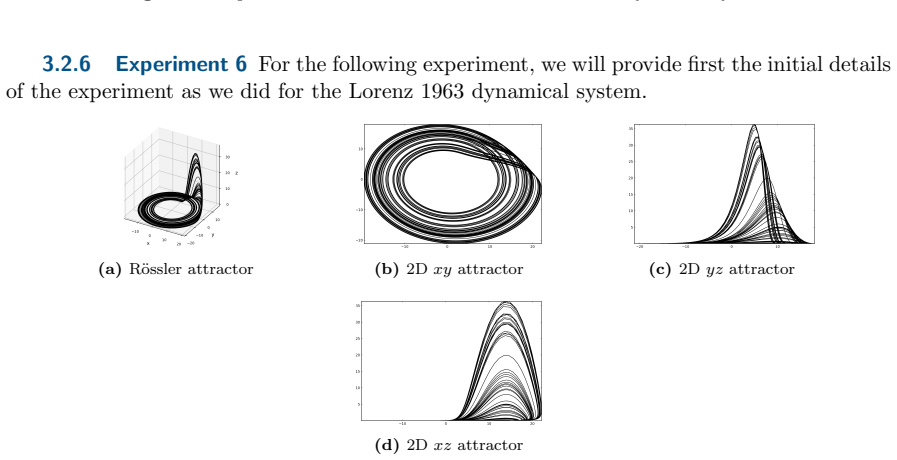
Summary. The paper presents a kernel-based extended dynamic mode decomposition (Lap-KeDMD) for sparse spatiotemporal reconstruction, together with an operator-theoretic analysis. The authors construct an RKHS H_L of holomorphic functions square-integrable with respect to a "Laplacian measure" (4.6), claim that the Laplacian kernel sections belong to H_L (Theorem 4.4), establish boundedness and compactness of Koopman operators with affine symbols on H_L (Theorems 5.3 and 6.5), contrast this with an alleged failure of closability for the GRBF kernel (Theorem 6.7), and derive approximation and faithfulness results for Koopman spectral measures and mode decompositions (Theorems 7.1 and 7.2). The paper also reports qualitative comparisons of Lap-KeDMD versus GRBF-KeDMD on seven datasets, including chaotic and PDE examples.
Significance. If correct, the paper would supply a principled operator-theoretic justification for using the Laplacian kernel in KeDMD, addressing a recognized open problem about closability of Koopman operators on RKHSs. The empirical scope (seven datasets, including Burgers equation, flow past a cylinder, Lorenz and Rössler attractors, traffic data, and NOAA SST anomalies) is a genuine strength, and the problem of connecting kernel choice to closable Koopman operators is timely and relevant. However, the central theoretical results contain multiple load-bearing errors: the Laplacian kernel sections are not established to be (and in general are not) holomorphic, so they need not lie in H_L; the closability proof in Theorem 6.5 uses an invalid change of variables and does not verify the norm-convergence condition required for closability; Theorem 7.1 uses a false identity about spectral-measure integrals; and Theorem 7.2 essentially restates the conclusion already built into Definition 2.4. Because these steps are load-bearing for the advertised operator-theoretic guarantee, the paper's central claim is not supported.
major comments (5)
- [§4.3, Theorem 4.4] The proof of Theorem 4.4 bounds only the L^2(μ_L) integral of |K^{1,σ}_exp(z,x)|^2 and never establishes that the function is holomorphic. For D=1, K^{1,σ}_exp(z,x)=exp(-|z-x|/σ) is not holomorphic in z on C, and the same failure occurs in higher dimensions, so the Laplacian kernel sections are not members of H_L as defined in (4.8). Consequently, the dictionary used in Algorithm 3.1 is not contained in the Hilbert space on which Theorems 5.3 and 6.5 apply, severing the proposed bridge from the RKHS theory to the Lap-KeDMD algorithm.
- [§6.2, Theorem 6.5] The proof's change of variables u=Az+b yields the factor exp(-||A^{-1}(u-b)||^2/σ) dV_D(u)/|det A|, but the next inequality replaces this with exp(-||Au||^2/σ) and then identifies the resulting integral with ||g_m||^2_{H_L}; this identification is false for a general invertible A because dμ_L(u) contains exp(-||u||/σ), not exp(-||Au||/σ). In addition, the proof does not establish closability: Lemma 6.4 requires that g_m→0 in H_L implies K_φ g_m→0 in H_L in norm, whereas (6.3) only shows pointwise convergence through the reproducing kernel. The theorem's conclusion is therefore not derived.
- [§7.2, Theorem 7.1, Eq. (7.8)] The identity [∫_D λ dV(λ) g](x) - [∫_D λ dV(λ) g](Ax) = [∫_D λ dV(λ) g](x-Ax) is false: the spectral measure integral is a linear operator applied to the function g, not a function of the evaluation point in such a way that argument differences can be pulled through. The subsequent steps also mix pointwise values with norms and treat |V(ρ(K_Ft))| as a scalar measure despite V being a projection-valued measure. The claimed bound (7.4)–(7.5) is therefore not proven.
- [§7.2, Theorem 7.2] The conclusion 𭟋Δ^(0,m)_{H_L} ≡ 0 is already asserted in Definition 2.4, Eq. (2.10), so Theorem 7.2 is a restatement rather than a proof. Moreover, the proof's claim that an infinite series summing to zero has partial sums equal to zero is incorrect; partial sums of a convergent series need not vanish, and the individual terms c_n[K^m_{F_t}ζ_n(x_0)-ζ_n(A^m x_0 + b∑ A^i)] need not be zero. The faithfulness result is thus true by construction, not by the argument given.
- [§6.2.1, Theorem 6.7] The proof concludes ∥K_φ g_m∥_{H_σ} = ∞ from an unbounded upper bound on the integral in (6.4). An upper bound that diverges does not imply that the actual norm diverges, so the assertion that K_φ g_m ∉ H_σ is not established. Furthermore, even if some sequence produced an infinite norm, closability failure would require exhibiting a sequence g_m→0 with K_φ g_m converging to a nonzero limit; no such sequence is given. The claimed contrast with the GRBF kernel is therefore unsupported.
minor comments (4)
- [Definition 2.5] The definition states X=∅, which contradicts the intended use of a nonempty input space throughout the paper; this should be X≠∅.
- [Table 3] The entry for W reads "Field of real, complex and whole numbers respectively"; the phrase "whole numbers" is unclear and should be replaced by the intended set (for example, natural numbers or integers).
- [§3.3] The experimental comparison is based on visual inspection of heat maps and error plots; no quantitative summary statistic (such as RMSE, mean absolute error, or correlation) is reported, which makes the claimed superiority of the Laplacian kernel difficult to assess.
- [Figure 1] The figure combines unexplained symbols (for example, the script F and the notation Δ^(0,m)_H) and is not self-contained; the caption should define all quantities shown.
Circularity Check
Faithful reconstruction is defined as zero and then re-proved as zero: Theorem 7.2 restates Definition 2.4, so the central 'theoretical justification' for Lap-KeDMD is circular.
-
self definitional
[Definition 2.4 (Section 2.2, Eqs. (2.8)-(2.10)) and Theorem 7.2 (Section 7.2, Eqs. (7.10)-(7.11))]
"𭟋∆(0,m) H := X n∈N cn [K m Ft ζn(x0)−ζn (A m x0 +b P m−1 i=0 A i )] ... When such a specific operator-theoretic quantification of the Koopman operator is determined subject to its existence over the Hilbert space H, then 𭟋∆(0,m) H = lim N→∞ PN 𭟋∆(0,m) H ≡ 0 (2.10) ... Then the faithful Koopman mode decomposition with respect to the RKHS HL is given as 𭟋∆(0,m) HL = P∞ n=1 cn [K m Ft ζn(x0)−ζn (A m x0 +b P m−1 i=0 A i )] (7.10) ... Lastly, lim N→∞ PN 𭟋∆(0,m) HL = 𭟋∆(0,m) HL ≡ 0. (7.11). Equating both equations with each other yields ... = 0."
Theorem 7.2's conclusion (7.11) is exactly the assertion (2.10) already built into Definition 2.4, and its formula (7.10) is the same series as (2.8). The proof does not derive the equality of the two Koopman-mode expansions; it 'equates' K_Ft^m ζ_n(x0) with ζ_n(A^m x0 + b Σ A^i), which is precisely the statement that each summand of 𭟋∆ vanishes. Closability/compactness of K_φ gives no reason for K_Ft and K_φ to act identically on ζ_n, nor that the same Koopman modes c_n apply to both expansions. Hence the advertised 'faithful reconstruction' is true by construction rather than by operator theory.
full rationale
The paper contains one genuinely circular, load-bearing step. Definition 2.4 defines the 'faithful' Koopman mode difference by formula (2.8) and then declares, in (2.10), that 𭟋∆(0,m)_H ≡ 0. Theorem 7.2 repeats that same formula as (7.10), repeats the same zero limit as (7.11), and 'proves' it by equating the two Koopman-mode series—an equality that is exactly the difference it is supposed to establish. Closability of K_φ gives no reason for K_Ft^m ζ_n(x0) to equal ζ_n(A^m x0 + bΣ A^i); that equality is assumed when the two expansions are equated. Thus the advertised guarantee that Laplacian-kernel ST reconstruction is 'faithful' is true by construction, not by the operator theory developed in Sections 5-6. Other claimed results are not circular in this sense. Theorem 6.5 is essentially the standard implication compact ⇒ closable, so it is trivial rather than derivational; Theorem 6.7 rests on an external result [29]; and the numerical comparisons are independent benchmarks. Self-citations in the references ([83], [84]) are not load-bearing. I note, without counting them as circularity, that Theorem 4.4 establishes only square-integrability of the Laplacian kernel section against dμ_L and never proves the holomorphy required by (4.8), that the change of variables in the proof of Theorem 6.5 is algebraically wrong, and that Theorem 7.1's choice of ϵ makes the bound vacuous; these are soundness defects, not circularity, but they mean the operator-theoretic bridge to Lap-KeDMD is not independently established.
Assumptions & free parameters
free parameters (2)
- Kernel bandwidth sigma =
1 (used in K1,1_exp and K2,1_exp)
- Affine symbol parameters A and b in phi(z)=Az+b =
unspecified (only constrained to 0<||A||_Frob<1, A invertible)
assumptions (6)
- domain assumption Underlying dynamical system has flow F_t and invariant Borel probability measure mu (Assumption 2.1)
- domain assumption Observables zeta_n belong to L2(Omega) intersect H_L and are Koopman eigenfunctions in both spaces (Section 7 setup)
- ad hoc to paper Koopman operator on H_L is bounded and compact for affine contraction symbols (Theorem 5.3, Note 5.2)
- ad hoc to paper The spectral integral representation integral lambda dV(lambda) applies to K_phiA on H_L in Theorem 7.1
- ad hoc to paper The Laplacian kernel K1,sigma_exp(.,x) belongs to H_L (Theorem 4.4)
- standard math Moore-Aronszajn and Bochner theorems
invented entities (1)
-
Hilbert space H_L with reproducing kernel K_sigma(z,w) = sinh(sqrt(<z,w>/sigma^2))/sqrt(<z,w>/sigma^2)
Cite this review
Pith. "Pith review of Kernel Dynamic Mode Decomposition For Sparse Reconstruction of Closable Koopman Operators." pith.science (2026). https://pith.science/paper/F24QI4BP
@misc{pith2026250506806,
  author       = {Pith},
  title        = {Pith review of: Kernel Dynamic Mode Decomposition For Sparse Reconstruction of Closable Koopman Operators},
  year         = {2026},
  howpublished = {\url{https://pith.science/paper/F24QI4BP}},
  note         = {Machine review of arXiv:2505.06806}
}
read the original abstract
Spatial temporal reconstruction of dynamical system is indeed a crucial problem with diverse applications ranging from climate modeling to numerous chaotic and physical processes. These reconstructions are based on the harmonious relationship between the Koopman operators and the choice of dictionary, determined implicitly by a kernel function. This leads to the approximation of the Koopman operators in a reproducing kernel Hilbert space (RKHS) associated with that kernel function. Data-driven analysis of Koopman operators demands that Koopman operators be closable over the underlying RKHS, which still remains an unsettled, unexplored, and critical operator-theoretic challenge. We aim to address this challenge by investigating the embedding of the Laplacian kernel in the measure-theoretic sense, giving rise to a rich enough RKHS to settle the closability of the Koopman operators. We leverage Kernel Extended Dynamic Mode Decomposition with the Laplacian kernel to reconstruct the dominant spatial temporal modes of various diverse dynamical systems. After empirical demonstration, we concrete such results by providing the theoretical justification leveraging the closability of the Koopman operators on the RKHS generated by the Laplacian kernel on the avenues of Koopman mode decomposition and the Koopman spectral measure. Such results were explored from both grounds of operator theory and data-driven science, thus making the Laplacian kernel a robust choice for spatial-temporal reconstruction.
Figures


Figures from the paper (24 more)




Reference graph
Works this paper leans on
-
[1]
Abramowitz, I
M. Abramowitz, I. A. Stegun, and D. Miller , Handbook of mathematical functions with formulas, graphs and mathematical tables (National Bureau of Standards Applied Mathematics Series No. 55) , (1965)
1965
-
[2]
R. J. Adler, The geometry of random fields , Wiley, 1981
1981
-
[3]
V. I. Arnol’d, Mathematical methods of classical mechanics, vol. 60, Springer Science & Business Media, 2013
2013
-
[4]
W. E. Arnoldi, The principle of minimized iterations in the solution of the matrix eigenvalue problem , Quarterly of Applied Mathematics, 9 (1951), pp. 17–29
1951
-
[5]
N. Aronszajn, Theory of reproducing kernels , Transactions of the American Mathematical Society, 68 (1950), pp. 337–404
work page 1950
-
[6]
P. J. Baddoo, B. Herrmann, B. J. McKeon, and S. L. Brunton, Kernel learning for robust Dynamic Mode Decomposition: Linear and Nonlinear disambiguation optimization , Proceedings of the Royal Society A, 478 (2022), p. 20210830
work page 2022
-
[7]
J. C. Baez, I. E. Segal, and Z. Zhou , Introduction to algebraic and constructive quantum field theory , vol. 56, Princeton University Press, 2014
work page 2014
-
[8]
V. Bargmann , On a Hilbert space of analytic functions and an associated integral transform part I , Communications on pure and applied mathematics, 14 (1961), pp. 187–214. 2follow Note 5.2. 34 HIMANSHU S. & NISHANT P. & J. NATHAN K
work page 1961
Show all 84 references
-
[9]
Bevanda, M
P. Bevanda, M. Beier, A. Lederer, S. Sosnowski, E. H ¨ullermeier, and S. Hirche , Koopman Kernel Regression, Advances in Neural Information Processing Systems, 36 (2024)
2024
-
[10]
S. L. Brunton, B. W. Brunton, J. L. Proctor, E. Kaiser, and J. N. Kutz , Chaos as an inter- mittently forced linear system, Nature communications, 8 (2017), p. 19
2017
-
[11]
S. L. Brunton and J. N. Kutz , Data-driven science and engineering: Machine learning, dynamical systems, and control, Cambridge University Press, 2022
2022
-
[12]
Budiˇsi´c, R
M. Budiˇsi´c, R. Mohr, and I. Mezi ´c, Applied Koopmanism, Chaos: An Interdisciplinary Journal of Nonlinear Science, 22 (2012)
2012
-
[13]
X. Chen, M. Lei, N. Saunier, and L. Sun , Low-rank autoregressive tensor completion for spatiotem- poral traffic data imputation , IEEE Transactions on Intelligent Transportation Systems, 23 (2021), pp. 12301–12310
2021
-
[14]
M. J. Colbrook , The Multiverse of Dynamic Mode Decomposition Algorithms , arXiv preprint arXiv:2312.00137, (2023)
2023 arXiv
-
[15]
M. J. Colbrook, Chapter 4 - The Multiverse of Dynamic Mode Decomposition Algorithms , in Numerical Analysis Meets Machine Learning, S. Mishra and A. Townsend, eds., vol. 25 of Handbook of Numerical Analysis, Elsevier, 2024, pp. 127–230, https://doi.org/https://doi.org/10.1016/...
2024 doi
-
[16]
J. B. Conway, A Course in Functional Analysis , vol. 96, Springer, 2019
2019
-
[17]
Z. Cui, K. Henrickson, R. Ke, and Y. Wang , Traffic graph convolutional recurrent neural network: A deep learning framework for network-scale traffic learning and forecasting , IEEE Transactions on Intelligent Transportation Systems, (2019)
2019
-
[18]
Z. Cui, R. Ke, and Y. Wang , Deep Bidirectional and Unidirectional LSTM Recurrent Neural Network for Network-wide Traffic Speed Prediction, arXiv preprint arXiv:1801.02143, (2018)
2018 arXiv
-
[19]
A. M. DeGennaro and N. M. Urban, Scalable Extended Dynamic Mode Decomposition using Random Kernel Approximation, SIAM Journal on Scientific Computing, 41 (2019), pp. A1482–A1499
2019
-
[20]
B. A. Dubrovin, A. T. Fomenko, and S. P. Novikov , Modern geometry—methods and applications: Part II: The geometry and topology of manifolds , vol. 104, Springer Science & Business Media, 2012
2012
-
[21]
Eisner, B
T. Eisner, B. Farkas, M. Haase, and R. Nagel, Operator theoretic aspects of ergodic theory, vol. 272, Springer, 2015
2015
-
[22]
G. E. Fasshauer, Meshfree approximation methods with MATLAB , vol. 6, World Scientific, 2007
2007
-
[23]
Freeman, D
D. Freeman, D. Giannakis, B. Mintz, A. Ourmazd, and J. Slawinska, Data assimilation in operator algebras, Proceedings of the National Academy of Sciences, 120 (2023), p. e2211115120
2023
-
[24]
Fujii and Y
K. Fujii and Y. Kawahara, Supervised Dynamic Mode Decomposition via Multitask Learning , Pattern Recognition Letters, 122 (2019), pp. 7–13
2019
-
[25]
Geifman, A
A. Geifman, A. Yadav, Y. Kasten, M. Galun, D. Jacobs, and B. Ronen, On the similarity between the Laplace and Neural Tangent Kernels , Advances in Neural Information Processing Systems, 33 (2020), pp. 1451–1461
2020
-
[26]
Geifman, A
A. Geifman, A. Yadav, Y. Kasten, M. Galun, D. Jacobs, and B. Ronen , On the Similarity between the Laplace and Neural Tangent Kernels , in Advances in Neural Information Processing Systems, H. Larochelle, M. Ranzato, R. Hadsell, M. Balcan, and H. Lin, eds., vol. 33, Curran Ass...
2020
-
[27]
Giannakis and S
D. Giannakis and S. Das, Extraction and prediction of coherent patterns in incompressible flows through space–time Koopman analysis, Physica D: Nonlinear Phenomena, 402 (2020), p. 132211
2020
-
[28]
Giraud and R
B. Giraud and R. Peschanski , On positive functions with positive Fourier transforms , Acta Physica Polonica B, 37 (2006), p. 331
2006
-
[29]
Gonzalez, M
E. Gonzalez, M. Abudia, M. Jury, R. Kamalapurkar, and J. A. Rosenfeld , The Kernel Per- spective on Dynamic Mode Decomposition , Transactions on Machine Learning Research, (2024), https://openreview.net/forum?id=sIR8xV7hGl
2024
-
[30]
Grigsby, Z
J. Grigsby, Z. Wang, N. Nguyen, and Y. Qi , Long-range transformers for dynamic spatiotemporal forecasting, arXiv preprint arXiv:2109.12218, (2021)
2021 arXiv
-
[31]
D. A. Haggerty, M. J. Banks, E. Kamenar, A. B. Cao, P. C. Curtis, I. Mezi ´c, and E. W. Hawkes, Control of soft robots with inertial dynamics , Science robotics, 8 (2023), p. eadd6864
2023
-
[32]
B. C. Hall, Quantum theory for Mathematicians , Springer, 2013. KERNEL EDMD FOR SPARSE RECONSTRUCTION OF CLOSABLE KOOPMAN OPERATORS 35
2013
-
[33]
Halmos, Bernoulli shifts , The American Mathematical Monthly, 84 (1977), pp
P. Halmos, Bernoulli shifts , The American Mathematical Monthly, 84 (1977), pp. 714–716
1977
-
[34]
Hasegawa, K
K. Hasegawa, K. Fukami, T. Murata, and K. Fukagata, CNN-LSTM based reduced order modeling of two-dimensional unsteady flows around a circular cylinder at different Reynolds numbers , Fluid Dynamics Research, 52 (2020), p. 065501
2020
-
[35]
He, C.-Y
Z. He, C.-Y. Chow, and J.-D. Zhang , STCNN: A Spatio-Temporal Convolutional Neural Network for Long-Term Traffic Prediction, in 2019 20th IEEE International Conference on Mobile Data Manage- ment (MDM), 2019, pp. 226–233, https://doi.org/10.1109/MDM.2019.00-53
2019 doi
-
[36]
T. L. Hill, An introduction to statistical thermodynamics , Courier Corporation, 1986
1986
-
[37]
L. Hui, S. Ma, and M. Belkin, Kernel machines beat deep neural networks on mask-based single-channel speech enhancement, Proc. Interspeech 2019, (2019), pp. 2748––2752
2019
-
[38]
Ikeda, I
M. Ikeda, I. Ishikawa, and Y. Sawano , Boundedness of composition operators on reproducing ker- nel Hilbert spaces with analytic positive definite functions , Journal of Mathematical Analysis and Applications, 511 (2022), p. 126048
2022
-
[39]
Ikeda, I
M. Ikeda, I. Ishikawa, and C. Schlosser , Koopman and Perron–Frobenius operators on reproducing kernel Banach spaces, Chaos: An Interdisciplinary Journal of Nonlinear Science, 32 (2022)
2022
-
[40]
Janson, J
S. Janson, J. Peetre, and R. Rochberg , Hankel Forms and the Fock space , Revista Matematica Iberoamericana, 3 (1987), pp. 61–138
1987
-
[41]
S. Klus, A. Bittracher, I. Schuster, and C. Sch ¨utte, A kernel-based approach to molecular con- formation analysis, The Journal of Chemical Physics, 149 (2018)
2018
-
[42]
S. Klus, P. Koltai, and C. Sch ¨utte, On the numerical approximation of the Perron-Frobenius and Koopman operator, Journal of Computational Dynamics, 3 (2016), pp. 51–79
2016
-
[43]
S. Klus, F. N ¨uske, and B. Hamzi , Kernel-based approximation of the Koopman generator and Schr¨ odinger operator, Entropy, 22 (2020), p. 722
2020
-
[44]
B. O. Koopman, Hamiltonian systems and transformation in Hilbert space , Proceedings of the National Academy of Sciences, 17 (1931), pp. 315–318
1931
-
[45]
B. O. Koopman and J. v. Neumann , Dynamical systems of continuous spectra , Proceedings of the National Academy of Sciences, 18 (1932), pp. 255–263
1932
-
[46]
K. Li, Y. Wang, P. Gao, G. Song, Y. Liu, H. Li, and Y. Qiao , Uniformer: Unified transformer for efficient spatiotemporal representation learning, arXiv preprint arXiv:2201.04676, (2022)
2022 arXiv
-
[47]
Q. Li, F. Dietrich, E. M. Bollt, and I. G. Kevrekidis, Extended Dynamic Mode Decomposition with dictionary learning: A data-driven adaptive spectral decomposition of the Koopman operator , Chaos: An Interdisciplinary Journal of Nonlinear Science, 27 (2017)
2017
-
[48]
Lorenz, Edward N , Deterministic nonperiodic flow , Journal of Atmospheric Sciences, 20 (1963), pp. 130–141
1963
-
[49]
Mezi´c, Spectral properties of dynamical systems, model reduction and decompositions , Nonlinear Dy- namics, 41 (2005), pp
I. Mezi´c, Spectral properties of dynamical systems, model reduction and decompositions , Nonlinear Dy- namics, 41 (2005), pp. 309–325
2005
-
[50]
Mezi´c, Spectrum of the Koopman operator, spectral expansions in functional spaces, and state-space geometry, Journal of Nonlinear Science, 30 (2020), pp
I. Mezi´c, Spectrum of the Koopman operator, spectral expansions in functional spaces, and state-space geometry, Journal of Nonlinear Science, 30 (2020), pp. 2091–2145
2020
-
[51]
Mezi ´c, Koopman operator, geometry, and learning of dynamical systems , Not
I. Mezi ´c, Koopman operator, geometry, and learning of dynamical systems , Not. Am. Math. Soc., 68 (2021), pp. 1087–1105
2021
-
[52]
Mezi´c and A
I. Mezi´c and A. Banaszuk , Comparison of systems with complex behavior , Physica D: Nonlinear Phe- nomena, 197 (2004), pp. 101–133
2004
-
[53]
Murata, K
T. Murata, K. Fukami, and K. Fukagata, Nonlinear Mode Decomposition with convolutional neural networks for fluid dynamics , Journal of Fluid Mechanics, 882 (2020), p. A13
2020
-
[54]
G. K. Pedersen, Analysis NOW, vol. 118, Springer Science & Business Media, 2012
2012
-
[55]
1, Springer, 2006
Rasmussen, Carl Edward and Williams, Christopher KI and others , Gaussian Processes for Machine Learning, vol. 1, Springer, 2006
2006
-
[56]
Reed, Methods of modern mathematical physics: Functional Analysis , Elsevier, 2012
M. Reed, Methods of modern mathematical physics: Functional Analysis , Elsevier, 2012
2012
-
[57]
J. A. Rosenfeld, R. Kamalapurkar, L. F. Gruss, and T. T. Johnson , Dynamic Mode Decom- position for Continuous Time Systems with the Liouville operator , Journal of Nonlinear Science, 32 (2022), pp. 1–30
2022
-
[58]
O. E. R ¨ossler, An equation for continuous chaos , Physics Letters A, 57 (1976), pp. 397–398
1976
-
[59]
C. W. Rowley, I. Mezi ´c, S. Bagheri, P. Schlatter, and D. S. Henningson , Spectral analysis of nonlinear flows, Journal of fluid mechanics, 641 (2009), pp. 115–127. 36 HIMANSHU S. & NISHANT P. & J. NATHAN K
2009
-
[60]
Rubanova, R
Y. Rubanova, R. T. Chen, and D. K. Duvenaud, Latent ordinary differential equations for irregularly- sampled time series , Advances in neural information processing systems, 32 (2019)
2019
-
[61]
Rudin, Functional Analysis 2nd ed, International Series in Pure and Applied Mathematics
W. Rudin, Functional Analysis 2nd ed, International Series in Pure and Applied Mathematics. McGraw- Hill, Inc., New York, (1991)
1991
-
[62]
Saad, Iterative methods for sparse linear systems , SIAM, 2003
Y. Saad, Iterative methods for sparse linear systems , SIAM, 2003
2003
-
[63]
I. H. Sarker , Deep learning: a comprehensive overview on techniques, taxonomy, applications and re- search directions, SN Computer Science, 2 (2021), p. 420
2021
-
[64]
P. J. Schmid , Dynamic Mode Decomposition of Numerical and Experimental Data , Journal of fluid mechanics, 656 (2010), pp. 5–28
2010
-
[65]
P. J. Schmid , Dynamic Mode Decomposition and its variants , Annual Review of Fluid Mechanics, 54 (2022), pp. 225–254
2022
-
[66]
Sch¨olkopf, The kernel trick for distances , Advances in Neural Information Processing Systems, 13 (2000)
B. Sch¨olkopf, The kernel trick for distances , Advances in Neural Information Processing Systems, 13 (2000)
2000
-
[67]
I. E. Segal, Mathematical problems of relativistic physics , vol. 2, American Mathematical Soc., 1963
1963
-
[68]
Singh, Machine Learning Application of Generalized Gaussian Radial Basis Function and Its Repro- ducing Kernel Theory, Mathematics, 12 (2024), p
H. Singh, Machine Learning Application of Generalized Gaussian Radial Basis Function and Its Repro- ducing Kernel Theory, Mathematics, 12 (2024), p. 829, https://www.mdpi.com/2227-7390/12/6/829
2024
-
[69]
M. L. Stein, Interpolation of spatial data: some theory for kriging , Springer Science & Business Media, 2012
2012
-
[70]
Steinwart and A
I. Steinwart and A. Christmann, Support Vector Machines, Springer Science & Business Media, 2008
2008
-
[71]
Steinwart, D
I. Steinwart, D. Hush, and C. Scovel, An explicit description of the reproducing kernel Hilbert spaces of Gaussian RBF Kernels , IEEE Transactions on Information Theory, 52 (2006), pp. 4635–4643
2006
-
[72]
Takesaki et al., Theory of operator algebras II , vol
M. Takesaki et al., Theory of operator algebras II , vol. 125, Springer, 2003
2003
-
[73]
J. H. Tu, C. W. Rowley, D. M. Luchtenburg, S. L. Brunton, and J. N. Kutz , ON DYNAMIC MODE DECOMPOSITION: THEORY AND APPLICATIONS, Journal of Computational Dynamics, 1 (2014), pp. 391–421
2014
-
[74]
G. E. Uhlenbeck and L. S. Ornstein , On the theory of the Brownian motion , Physical review, 36 (1930), p. 823
1930
-
[75]
Walters, An introduction to Ergodic Theory , vol
P. Walters, An introduction to Ergodic Theory , vol. 79, Springer Science & Business Media, 2000
2000
-
[76]
M. O. Williams, I. G. Kevrekidis, and C. W. Rowley, A data–driven approximation of the Koopman operator: Extending Dynamic Mode Decomposition, Journal of Nonlinear Science, 25 (2015), pp. 1307– 1346
2015
-
[77]
B. Yan, H. Peng, J. Fu, D. Wang, and H. Lu, Learning spatio-temporal transformer for visual tracking, in Proceedings of the IEEE/CVF international conference on computer vision, 2021, pp. 10448–10457
2021
-
[78]
S. Ye, Z. Zhang, X. Song, Y. Wang, Y. Chen, and C. Huang , A flow feature detection method for modeling pressure distribution around a cylinder in non-uniform flows by using a convolutional neural network, Scientific reports, 10 (2020), p. 4459
2020
-
[79]
C. Yu, X. Ma, J. Ren, H. Zhao, and S. Yi , Spatio-temporal graph transformer networks for pedestrian trajectory prediction, in Computer Vision–ECCV 2020: 16th European Conference, Glasgow, UK, August 23–28, 2020, Proceedings, Part XII 16, Springer, 2020, pp. 507–523
2020
-
[80]
H. M. Zhang, B. Huang, J. H. Lawrimore, M. J. Menne, and T. M. Smith , NOAA Global Sur- face Temperature Dataset (NOAAGlobalTemp), Version 5.0 , NOAA National Centers for Environ- mental Information, (2019), https://doi.org/10.25921/9qth-2p70;https://www.ncei.noaa.gov/data/ no...
2019 doi
-
[81]
S. Zhou, W. Shen, D. Zeng, M. Fang, Y. Wei, and Z. Zhang , Spatial–temporal convolutional neural networks for anomaly detection and localization in crowded scenes , Signal Processing: Image Com- munication, 47 (2016), pp. 358–368, https://doi.org/https://doi.org/10.1016/j.imag...
2016 doi
-
[82]
Zhu, Analysis on Fock Spaces, vol
K. Zhu, Analysis on Fock Spaces, vol. 263, Springer Science & Business Media, 2012
2012
-
[83]
Panda, M Giselle
N. Panda, M Giselle. Fern ´andez-Godino, H. Godinez, and C. Dawson , A data-driven non- linear assimilation framework with neural networks , Computational Geosciences, Springer, 2021, 25, pp. 233–242
2021
-
[84]
Panda, J H
N. Panda, J H. Chaudhry, N. Klein, J. Carzon and T. Butler, Local Stochastic Sensitivity Analysis For Dynamical Systems Proceedings of the 28th International Conference on Artificial Intelligence and Statistics, PMLR 258:4195-4203
Reviewed August 15, 2026 · model on record in the stance chip above.
Discussion (0). Continue with ORCID to comment.