Rate of Convergence for a Nonlocal-to-local Limit in One Dimension

Charles Elbar; Jakub Skrzeczkowski; Jos\'e A. Carrillo; Stefano Fronzoni

REVIEW 1 major objections 5 minor 28 references

Rate of Convergence for a Nonlocal-to-local Limit in One Dimension

T0 review · 1 major / 5 minor · reviewed 2026-08-15 · deepseek-v4-flash

Challenge this review Re-run · record.json Download PDF Read on arXiv ↗ Review JSON

Pith's one-line read In one dimension, the nonlocal porous medium equation converges to the local equation at rate $O(\sqrt{\varepsilon})$ in 2-Wasserstein distance for initial data in $\mathcal{P}_2(\mathbb{R})\cap L^\infty(\mathbb{R})$.

desk verdict Clean EVI proof of the √ε rate on the whole line with L1∩L∞ data; the rate is pre-existing, but the method and assumptions are new, and the paper is sound once the EVI comparison lemma is stated explicitly. read the letter →

arxiv 2505.07015 v1 pith:RGOPRDPG submitted 2025-05-11 math.AP cs.NAmath.NA

José A. Carrillo , Charles Elbar , Stefano Fronzoni , Jakub Skrzeczkowski This is my paper · ORCID

classification math.APcs.NAmath.NA MSC 35A1535Q7035B4065M08

keywords nonlocal-to-locallimitporousmediumequationWassersteindistancegradientflowsevolutionaryvariationalinequalityblobmethodfinitevolumerateofconvergence

verification ladder T0 review T1 audit T2 compute T3 formal

The pith

A machine-rendered reading of the paper's core claim, the machinery that carries it, and where it could break.

The reading

This paper proves that in one spatial dimension the solution of the nonlocal porous-medium equation $\partial_t u^\varepsilon-\partial_x(u^\varepsilon\partial_x W^\varepsilon*u^\varepsilon)=0$ converges to the solution of the quadratic porous medium equation $\partial_t u-\partial_{xx}(u^2/2)=0$ at a quantified rate: the $2$-Wasserstein distance satisfies $W_2(u^\varepsilon(t,\cdot),u(t,\cdot))\le C\sqrt{\varepsilon}$ for every $t\in[0,T]$, whenever the initial datum lies in $\mathcal{P}_2(\mathbb{R})\cap L^\infty(\mathbb{R})$. The constant $C$ depends only on the initial datum, the time horizon, and the kernel, never on $\varepsilon$. The proof is short, combining the evolutionary variational inequality characterization of both gradient flows with uniform a priori estimates. The result matters because the nonlocal equation underlies deterministic particle or blob approximations of the porous medium equation, and the rate makes the approximation error explicit without any differentiability assumption on the initial datum.

What carries the argument

The machinery is the evolutionary variational inequality (EVI), a gradient-flow characterization asserting that for every competitor $\sigma$ in the domain, $F(\mu_t)+\frac12\frac{d}{dt}W_2^2(\mu_t,\sigma)\le F(\sigma)$ for almost every $t$. Both the nonlocal and local equations are EVI gradient flows for their respective energies, and the proof combines the two EVIs with the elliptic identity $-\varepsilon^2\partial_{xx}W^\varepsilon+W^\varepsilon=\delta_0$ and the imported estimate that $\varepsilon\partial_{xx}(W^\varepsilon*u^\varepsilon)$ is uniformly bounded in $L^2((0,T)\times\mathbb{R})$. The identity translates the $L^2$ distance between $u^\varepsilon$ and its mollification into $\varepsilon^2$ times a second derivative, and the boundedness of that second derivative is what converts the energy error into an $O(\varepsilon)$ term, ultimately an $O(\sqrt{\varepsilon})$ Wasserstein rate.

What would settle it

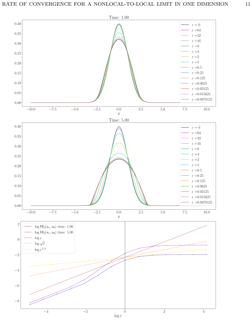
Solve (1.1) and (1.3) numerically with $\Delta x\le\varepsilon$ for a Gaussian initial datum and plot $W_2(u^\varepsilon,u)/\sqrt{\varepsilon}$; if this ratio is unbounded as $\varepsilon\to0$ for any fixed time $t>0$, the claimed constant $C$ in Theorem 1.1 cannot exist.

Watch

Extended reading notes

Core claim

The paper's central claim is that the nonlocal-to-local limit has order $\sqrt{\varepsilon}$ in $W_2$, under minimal integrability assumptions. The mechanism is a comparison of two Wasserstein gradient flows: the nonlocal energy $E^\varepsilon[\rho]=\frac12\int_\mathbb{R}\rho\,W^\varepsilon*\rho\,dx$ and the local energy $E[\rho]=\frac12\int_\mathbb{R}\rho^2\,dx$ are both $\lambda$-geodesically convex with $\lambda=0$, so their flows are characterized by the same evolutionary variational inequality. Inserting one flow as the competitor in the other's inequality and adding the two inequalities bounds $\frac12\frac{d}{dt}W_2^2(u^\varepsilon,u)$ by the energy differences $E^\varepsilon(u)-E(u)$ and $E(u^\varepsilon)-E^\varepsilon(u^\varepsilon)$. The first difference is nonpositive by the elementary inequality $u(x)u(y)\le \frac12u(x)^2+\frac12u(y)^2$; the second is bounded by $\frac12\|u^\varepsilon\|_{L^2}\|u^\varepsilon-u^\varepsilon*W^\varepsilon\|_{L^2}$, which via the identity $u^\varepsilon-u^\varepsilon*W^\varepsilon=-\varepsilon^2\partial_{xx}(W^\varepsilon*u^\varepsilon)$ and the a priori estimate $\|\varepsilon\partial_{xx}(W^\varepsilon*u^\varepsilon)\|_{L^2}\le C$ becomes $C\varepsilon$. Integrating in time yields the $\sqrt{\varepsilon}$ rate.

Load-bearing premise

The argument assumes an unstated comparison principle that turns the two variational inequalities into a bound on how fast the two flows separate, and it imports a second-order regularity estimate for the nonlocal solutions; if either ingredient gives way, the proof collapses.

Editorial extensions

If this is right

For every initial datum in $\mathcal{P}_2(\mathbb{R})\cap L^\infty(\mathbb{R})$, the blob/particle approximation to the quadratic porous medium equation converges in $W_2$ at rate $O(\sqrt{\varepsilon})$, uniformly on any finite time interval.
The rate is global in $\varepsilon$: the bound $C\sqrt{\varepsilon}$ holds for all $\varepsilon>0$, not only in an asymptotic regime, because no restriction on $\varepsilon$ is imposed in the proof.
No derivative or higher regularity of the initial datum is needed; finite second moment, $L^\infty$ boundedness, and integrability suffice.
The numerical simulations indicate that for small $\varepsilon$ the observed rate is closer to $\varepsilon$ than to $\sqrt{\varepsilon}$, so the theorem's bound may not be sharp in the small-$\varepsilon$ regime while remaining the best global-in-$\varepsilon$ estimate.
Under no-flux boundary conditions, the numerical experiments suggest the rate can degrade to $\sqrt{\varepsilon}$ once the solution touches the boundary, showing that boundary interaction can erode the faster rate seen on the whole line.

Reading between the lines

Editorial extensions of the paper, not claims the author makes directly.

The unstated comparison lemma for $\lambda=0$ EVI gradient flows is the real workhorse; stated explicitly, the same two-line energy-difference argument would give rates for any pair of nonlocal/local gradient flows that admit a matching second-order estimate.
The numerical transition from $\varepsilon$ to $\sqrt{\varepsilon}$ under no-flux boundaries hints at a boundary-layer mechanism: one could test whether the $W_2$ error is dominated by a layer of width $\varepsilon$ near the boundary, in which case interior estimates might still be linear in $\varepsilon$.
Estimate (D) is imported rather than proved; deriving it from scratch for more general kernels, or finding a kernel for which it fails, would delimit exactly how far the EVI-comparison method extends.
The one-dimensional proof uses monotonicity of optimal transport maps to show geodesic convexity of $E^\varepsilon$; a higher-dimensional analogue would need a different convexity argument, consistent with the alternative route used in the broader recent treatment of the problem.

Share X Bluesky LinkedIn Reddit HN

Signed reviews

No signed human review yet.

Editorial analysis

A structured set of objections, weighed in public.

Desk editor's note, referee report, and a circularity audit.

Desk Editor's Note

read the letter

The short version: this is a nice, compact paper proving a √ε Wasserstein rate for a particular nonlocal-to-local limit in 1D via EVI gradient flow ideas. The rate itself was already available from Amassad–Zhou for a broader kernel class, so the novelty is not the rate. What is genuinely new is the relaxation of the initial datum to P2∩L∞ on the whole line (no W^{1,∞} on the torus) and a much simpler proof technique. The numerical section adds some evidence about sharpness, but it overstates what it shows. The analytic proof is essentially correct. The stress-test note is right that the combination of the two EVIs is not fully justified as written. The EVI holds for every fixed test measure but with an exceptional set that can depend on the test; to set s=t one needs an explicit comparison/chain-rule argument, or a justification via absolute continuity and approximation by a countable dense set. That is a genuine but small gap, and it is repairable. The referee should ask for it to be stated. Everything else checks out: estimate (D) imported from Perthame–Vauchelet et al. supplies the ε factor, and the log-entropy sketch in Proposition 2.1 is plausible and supported by the cited work. Minor issues: the paper says the numerics 'demonstrate' that the estimate is the best global-in-ε estimate. That is too strong. The experiments show linear behavior for small ε and slower behavior for large ε, which suggests sharpness, but a few finite-volume runs on bounded domains with specific initial data do not demonstrate it. Also, the forthcoming work [6] is cited as confirmation, but it is not evidence yet. The paper is honest about the comparison to Amassad–Zhou, which it cites clearly. Who is this for? People working on blob methods, nonlocal approximations of degenerate diffusion, or gradient flows in Wasserstein space. It is a clean proof-of-concept that the EVI route gives rates under weak assumptions. It deserves a serious referee. I would recommend acceptance after minor revision: state the missing lemma, and temper the numerics language.

Referee Report

1 major / 5 minor

Summary. The paper proves a quantitative convergence rate for the nonlocal-to-local limit in one dimension between the nonlocal porous-medium-type equation ∂t uε = ∂x(uε ∂x(Wε ∗ uε)), with Wε the exponentially decaying Laplace kernel, and the local quadratic porous medium equation ∂t u = ∂xx(u²/2). The main result, Theorem 1.1, asserts that W2(uε(t,·), u(t,·)) ≤ C√ε for all t ∈ [0,T] under only u0 ∈ P2(R) ∩ L∞(R). The proof combines the Evolutionary Variational Inequality characterization of both gradient flows with uniform a priori estimates imported from [23,24]; a finite-volume numerical section illustrates the rate and suggests possible improvements for small ε. The paper is short, clearly written, and the overall strategy is attractive, but the central EVI comparison step is not fully justified as written.

Significance. If the gap described below is repaired, this is a clean and useful result: it obtains the √ε rate in the Wasserstein distance under weaker regularity assumptions than the concurrent work [1] (no W^{1,∞} condition and no torus), and the EVI strategy is transparent. The imported a priori estimate (D) of Proposition 2.1 is adequately supported by the log-entropy computation sketched there, and the finite-volume experiments, while not a proof, are consistent with the theorem. The main missing piece is a standard but unstated comparison lemma for two EVI gradient flows; once supplied, the proof should be complete.

major comments (1)

[Section 2.3, Eqs. (2.3)-(2.4)] The step 'Combining (2.3) and (2.4)' is the central step of the proof and is not justified as written. First, Eq. (2.4) differentiates W2^2(u(t,·), uε(s,·)) with respect to t, whereas the needed inequality differentiates H(t,s)=W2^2(uε(t,·),u(s,·)) with respect to the second argument s; the displayed derivative variable appears to be a typo. Second, even after that correction, applying Theorem 2.3 with the time-dependent test measures u(s) and uε(t) requires a comparison lemma for two EVI gradient flows: for a.e. t, (1/2)(d/dt)W2^2(μ_t,ν_t) ≤ F(ν_t)-F(μ_t)+G(μ_t)-G(ν_t), with F,G the two energy functionals. This lemma is not stated or cited, and the exceptional-null-set issue for test measures depending on the evolution variable must be addressed, for example by using absolute continuity and approximation by a countable dense subset of the domain. Since the final bound relies entirely on this inequality, Theorem 1.1 is not fully proved as written; the gap is standard and likely repairable.

minor comments (5)

[Section 2.1, Eq. (2.1)] The displayed identity for the energy dissipation is missing the right-hand side; it should be written as an equality to 0.
[Section 2.2, Theorem 2.3] The paper does not explicitly verify the hypotheses of the quoted characterization, namely properness, lower semicontinuity and λ-geodesic convexity of E and Eε, and density of their domains. These are standard for the two functionals considered, but a brief verification would make the application self-contained.
[Section 3, Eq. (3.1b)] The numerical upwind flux appears to contain an index error: the second term uses v^-_{i-1/2} and (u_i^ε)_L at the interface i+1/2; the standard upwind reconstruction would use v^-_{i+1/2} and the left reconstructed value of the neighboring cell. Please check and correct.
[Section 4.1] The statement that the numerical experiments demonstrate that (1.4) is 'the best, global in ε estimate' goes beyond what finite-volume experiments can establish; it should be phrased as an observation or conjecture, particularly since the improved small-ε rate is deferred to the forthcoming paper [6]. The comparison of exponents in the sentence containing 'ε<√ε<ε^{1/4}' is also confusing for ε>1 and should be clarified.
[Proposition 2.4] The geodesic-convexity proof is written for the case where the optimal transport is given by a map T, i.e. for absolutely continuous ρ0; since Theorem 2.3 is applied on all of P2(R), a sentence on approximation of general measures by absolutely continuous ones is needed.

Circularity Check

0 steps flagged · score 0.0 of 10

No significant circularity: the √ε bound follows from independent a priori estimates plus the standard EVI characterization; the self-citations are not load-bearing.

full rationale

The central claim of Theorem 1.1 is derived from two genuinely independent ingredients: (i) the a priori estimates (A)–(E) of Proposition 2.1, imported from the external references [23,24] (Perthame et al.) and sketched in the paper, and (ii) the EVI characterization of gradient flows quoted from the external textbook [3]. The geodesic convexity of E_ε needed for the EVI is actually proved in Proposition 2.4; the citation [11] points to an earlier argument but is not load-bearing because the proof is written out in the text. The final step uses only the elementary inequality E_ε ≤ E and estimate (D), which gives the ε factor through the identity u_ε − W_ε * u_ε = −ε² ∂_xx(W_ε * u_ε). No fitted parameter is renamed as a prediction, and no equation is defined in terms of the target rate. The only caveat is a technical gap, not circularity: the passage from the two EVIs (2.3) and (2.4) to the differential inequality for (1/2) d/dt W₂²(u_ε(t), u(t)) is asserted without stating the required comparison/chain-rule lemma. That lemma is a standard consequence of the EVI and a.e. absolute continuity of the two flows, and it does not presuppose the desired bound. The forward reference [6] concerns an improved rate for small ε and is explicitly not used in the proof of Theorem 1.1. I therefore find no circular step.

Assumptions & free parameters 0 free parameters · 4 assumptions · 0 invented entities

No free parameters are fitted in the analytical result; the constant C is generic. The proof depends on standard gradient flow theory, prior a priori estimates, and the specific kernel's convexity, all listed above. No new entities are postulated.

assumptions (4)

standard math EVI characterization theorem for λ-geodesically convex functionals on P2(R) (Theorem 2.3, from [3, Theorem 11.1.4]).
Main tool; used to obtain inequalities (2.3) and (2.4).
domain assumption The PDE solutions uε and u are the unique EVI gradient flows of Eε and E with λ=0.
Invoked through [2, Prop 3.28, 3.38] in Section 2.3; needed to write the EVIs for the two equations.
standard math A priori estimates (A)-(E) of Proposition 2.1 hold for solutions of (1.1).
Recalled from [23,24] with a sketch; estimate (D) is load-bearing because it produces the ε factor.
standard math Geodesic convexity of Eε in 1D for kernels convex on each half-line (Proposition 2.4).
Proven using monotone optimal transport maps, following [11, Prop 2.7]; restricts the method to kernels like W(x)=1/2 e^{-|x|}.

how reviews work

0 comments

Cite this review

Pith. "Pith review of Rate of Convergence for a Nonlocal-to-local Limit in One Dimension." pith.science (2026). https://pith.science/paper/RGOPRDPG

@misc{pith2026250507015,
  author       = {Pith},
  title        = {Pith review of: Rate of Convergence for a Nonlocal-to-local Limit in One Dimension},
  year         = {2026},
  howpublished = {\url{https://pith.science/paper/RGOPRDPG}},
  note         = {Machine review of arXiv:2505.07015}
}

read the original abstract

We consider a nonlocal approximation of the quadratic porous medium equation where the pressure is given by a convolution with a mollification kernel. It is known that when the kernel concentrates around the origin, the nonlocal equation converges to the local one. In one spatial dimension, for a particular choice of the kernel, and under mere assumptions on the initial condition, we quantify the rate of convergence in the 2-Wasserstein distance. Our proof is very simple, exploiting the so-called Evolutionary Variational Inequality for both the nonlocal and local equations as well as a priori estimates. We also present numerical simulations using the finite volume method, which suggests that the obtained rate can be improved - this will be addressed in a forthcoming work.

Figures

Figures reproduced from arXiv: 2505.07015 by the authors.

**Figure 2.** Porous medium equation versus blob method: order of convergence for W2(uε, u0), u0 solution of (1.3) and uε solution of (1.1). The computational domain is Ω = (−10, 10), u 0 (x) = (1/ √ 2π) exp(−|x| 2/2) is the initial datum, a uniform grid of N = 212 cells was used with ∆t = 0.01 [PITH_FULL_IMAGE:figures/full_fig_p011_2.png] view at source ↗

**Figure 3.** Porous medium equation and blob method: order of convergence for W2(uε, u0), u0 solution of (1.3) and uε solution of (1.1). The computational domain Ω = (−3, 3), u 0 (x) = (1 − x 2 )+ is the initial datum, a uniform grid of N = 210 cells with ∆t = 0.01 was used, periodic boundary conditions were imposed [PITH_FULL_IMAGE:figures/full_fig_p012_3.png] view at source ↗

Figures from the paper (4 more)

**Figure 4.** Figure 4: Porous medium equation and blob method: order of convergence for W2(uε, u0), u0 solution of (1.3) and uε solution of (1.1). The computational domain is Ω = (−3, 3), u 0 (x) = (1 − x 2 )+ is the initial datum, a uniform grid of N = 210 cells was used with ∆t = 0.01, no…

**Figure 5.** Figure 5: Porous medium Fokker-Planck equation and blob method: order of convergence for W2(uε, u0), u0 solution of (3.6) and uε solution of (3.7). The computational domain is Ω = (−20, 20), u 0 (x) = 1/|Ω|+ 10 is the initial datum, a uniform grid of N = 213 cells was used with …

**Figure 6.** Figure 6: Porous medium equation and blob method: order of convergence for W2(uε, u0), u0 (solution of (3.6)) and uε (solution of (3.7)). The computational domain is Ω = (−10, 10), u 0 (x) = u(x, 0), the initial datum, is generated using random values on a uniform grid of N = 2…

**Figure 7.** Figure 7: Porous medium equation and blob method: u (solution of (3.6)) and uε (solution of (3.7)) for ε = 1. Ω = (−20, 20), u 0 (x) = u(x, 0) initial datum generated using random values on a uniform grid of N = 29 cells, ∆t = 0.01 [PITH_FULL_IMAGE:figures/full_fig_p018_7.png]

Discussion (0). Continue with ORCID to comment.

Reference graph

Works this paper leans on

28 extracted references · 19 canonical work pages

[6]

Carrillo, P

J. Carrillo, P. Gwiazda, and J. Skrzeczkowski. A new semigroup formula for the Wasserstein distance between two Wasserstein gradient flows.In preparation, 2025

work page 2025
[1]

A deterministic particle method for the porous media equation

A. Amassad and D. Zhou. A deterministic particle method for the porous media equation.arXiv preprint arXiv:2501.18745, 2025

work page Pith review arXiv 2025
[2]

Ambrosio and N

L. Ambrosio and N. Gigli. A user’s guide to optimal transport. InModelling and optimisation of flows on networks, volume 2062 ofLecture Notes in Math., pages 1–155. Springer, Heidelberg, 2013

work page 2013
[3]

Ambrosio, N

L. Ambrosio, N. Gigli, and G. Savaré.Gradient flows in metric spaces and in the space of probability measures. Lectures in Mathematics ETH Zürich. Birkhäuser Verlag, Basel, second edition, 2008

2008
[4]

Bailo, J

R. Bailo, J. A. Carrillo, S. Fronzoni, and D. Gómez-Castro. A finite-volume scheme for fractional diffusion on bounded domains.European Journal of Applied Mathematics, page 1–21, 2024

work page 2024
[5]

Burger and A

M. Burger and A. Esposito. Porous medium equation and cross-diffusion systems as limit of nonlocal interaction.Nonlinear Anal., 235:Paper No. 113347, 30, 2023

2023
[7]

J. A. Carrillo, A. Chertock, and Y. Huang. A finite-volume method for nonlinear nonlocal equations with a gradient flow structure.Commun. Comput. Phys., 17(1):233–258, 2015

work page 2015
[8]

J. A. Carrillo, K. Craig, and F. S. Patacchini. A blob method for diffusion.Calc. Var. Partial Differential Equations, 58(2):Paper No. 53, 53, 2019

2019

Show all 28 references

[9]

J. A. Carrillo, A. Esposito, J. Skrzeczkowski, and J. S.-H. Wu. Nonlocal particle approximation for linear and fast diffusion equations.arXiv preprint arXiv:2408.02345, 2024

2024 arXiv
[10]

J. A. Carrillo, A. Esposito, and J. S.-H. Wu. Nonlocal approximation of nonlinear diffusion equations. Calc. Var. Partial Differential Equations, 63(4):Paper No. 100, 44, 2024

2024
[11]

Math., 231(1):306–327, 2012

J.A.Carrillo, L.C.F.Ferreira, andJ.C.Precioso.Amass-transportationapproachtoaonedimensional fluid mechanics model with nonlocal velocity.Adv. Math., 231(1):306–327, 2012

2012
[12]

Craig, M

K. Craig, M. Jacobs, and O. Turanova. Nonlocal approximation of slow and fast diffusion.J. Differential Equations, 426:782–852, 2025. 20 JOSÉ A. CARRILLO, CHARLES ELBAR, STEF ANO FRONZONI, AND JAKUB SKRZECZKOWSKI

2025
[13]

David, T

N. David, T. Dębiec, M. Mandal, and M. Schmidtchen. A degenerate cross-diffusion system as the inviscid limit of a nonlocal tissue growth model.SIAM J. Math. Anal., 56(2):2090–2114, 2024

2024
[14]

David and B

N. David and B. Perthame. Free boundary limit of a tumor growth model with nutrient.J. Math. Pures Appl. (9), 155:62–82, 2021

2021
[15]

Doumic, S

M. Doumic, S. Hecht, B. Perthame, and D. Peurichard. Multispecies cross-diffusions: from a nonlocal mean-field to a porous medium system without self-diffusion.J. Differential Equations, 389:228–256, 2024

2024
[16]

Dębiec, B

T. Dębiec, B. Perthame, M. Schmidtchen, and N. Vauchelet. Incompressible limit for a two-species model with coupling through Brinkman’s law in any dimension.J. Math. Pures Appl. (9), 145:204–239, 2021

2021
[17]

Dębiec and M

T. Dębiec and M. Schmidtchen. Incompressible limit for a two-species tumour model with coupling through Brinkman’s law in one dimension.Acta Appl. Math., 169:593–611, 2020

2020
[18]

Elbar and J

C. Elbar and J. Skrzeczkowski. On the inviscid limit connecting Brinkman’s and Darcy’s models of tissue growth with nonlinear pressure.J. Math. Fluid Mech., 27(2):Paper No. 28, 14, 2025

2025
[19]

Lions and S

P.-L. Lions and S. Mas-Gallic. Une méthode particulaire déterministe pour des équations diffusives non linéaires.C. R. Acad. Sci. Paris Sér. I Math., 332(4):369–376, 2001

2001
[20]

Mellet, B

A. Mellet, B. Perthame, and F. Quirós. A Hele-Shaw problem for tumor growth.J. Funct. Anal., 273(10):3061–3093, 2017

2017
[21]

Oelschläger

K. Oelschläger. Large systems of interacting particles and the porous medium equation.J. Differential Equations, 88(2):294–346, 1990

1990
[22]

Perthame, F

B. Perthame, F. Quirós, and J. L. Vázquez. The Hele-Shaw asymptotics for mechanical models of tumor growth.Arch. Ration. Mech. Anal., 212(1):93–127, 2014

2014
[23]

Perthame, M

B. Perthame, M. Tang, and N. Vauchelet. Traveling wave solution of the Hele-Shaw model of tumor growth with nutrient.Math. Models Methods Appl. Sci., 24(13):2601–2626, 2014

2014
[24]

Perthame and N

B. Perthame and N. Vauchelet. Incompressible limit of a mechanical model of tumour growth with viscosity.Philos. Trans. Roy. Soc. A, 373(2050):20140283, 16, 2015

2015
[25]

Santambrogio.Optimal transport for applied mathematicians, volume 87 ofProgress in Nonlinear Differential Equations and their Applications

F. Santambrogio.Optimal transport for applied mathematicians, volume 87 ofProgress in Nonlinear Differential Equations and their Applications. Birkhäuser/Springer, Cham, 2015. Calculus of variations, PDEs, and modeling

2015
[26]

M. Tang, N. Vauchelet, I. Cheddadi, I. Vignon-Clementel, D. Drasdo, and B. Perthame. Composite waves for a cell population system modeling tumor growth and invasion.Chinese Ann. Math. Ser. B, 34(2):295–318, 2013

2013
[27]

J. M. Urbano.The method of intrinsic scaling, volume 1930 ofLecture Notes in Mathematics. Springer- Verlag, Berlin, 2008. A systematic approach to regularity for degenerate and singular PDEs. RATE OF CONVERGENCE FOR A NONLOCAL-TO-LOCAL LIMIT IN ONE DIMENSION 21

1930
[28]

Villani.Topics in optimal transportation, volume 58 ofGraduate Studies in Mathematics

C. Villani.Topics in optimal transportation, volume 58 ofGraduate Studies in Mathematics. American Mathematical Society, Providence, RI, 2003. José A. Carrillo:Mathematical Institute, University of Oxford, Woodstock Road, Oxford, OX2 6GG, United Kingdom Email address:carrillo@...

2003

Pith tools

Reviewed August 15, 2026 · model on record in the stance chip above.

[1] [6]

Carrillo, P

J. Carrillo, P. Gwiazda, and J. Skrzeczkowski. A new semigroup formula for the Wasserstein distance between two Wasserstein gradient flows.In preparation, 2025

work page 2025

[2] [1]

A deterministic particle method for the porous media equation

A. Amassad and D. Zhou. A deterministic particle method for the porous media equation.arXiv preprint arXiv:2501.18745, 2025

work page Pith review arXiv 2025

[3] [2]

Ambrosio and N

L. Ambrosio and N. Gigli. A user’s guide to optimal transport. InModelling and optimisation of flows on networks, volume 2062 ofLecture Notes in Math., pages 1–155. Springer, Heidelberg, 2013

work page 2013

[4] [3]

Ambrosio, N

L. Ambrosio, N. Gigli, and G. Savaré.Gradient flows in metric spaces and in the space of probability measures. Lectures in Mathematics ETH Zürich. Birkhäuser Verlag, Basel, second edition, 2008

2008

[5] [4]

Bailo, J

R. Bailo, J. A. Carrillo, S. Fronzoni, and D. Gómez-Castro. A finite-volume scheme for fractional diffusion on bounded domains.European Journal of Applied Mathematics, page 1–21, 2024

work page 2024

[6] [5]

Burger and A

M. Burger and A. Esposito. Porous medium equation and cross-diffusion systems as limit of nonlocal interaction.Nonlinear Anal., 235:Paper No. 113347, 30, 2023

2023

[7] [7]

J. A. Carrillo, A. Chertock, and Y. Huang. A finite-volume method for nonlinear nonlocal equations with a gradient flow structure.Commun. Comput. Phys., 17(1):233–258, 2015

work page 2015

[8] [8]

J. A. Carrillo, K. Craig, and F. S. Patacchini. A blob method for diffusion.Calc. Var. Partial Differential Equations, 58(2):Paper No. 53, 53, 2019

2019