REVIEW 1 major objections 5 minor 15 references
Applying the ACE2 Emulator to SST Green's Functions for the E3SMv3 Global Atmosphere Model
T0 review · 1 major / 5 minor · reviewed 2026-08-15 · deepseek-v4-flash
Pith's one-line read A machine-learning emulator reproduces a climate model's sea-surface-temperature response maps for top-of-atmosphere radiation about 100 times faster, with the largest bias in the tropical eastern Pacific.
desk verdict A careful, honest controlled comparison of ACE2 vs EAMv3 on GFMIP Green's functions; the qualitative conclusion holds, but the significance claims lean on an under-verified uniform variability assumption. read the letter →
The pith
A machine-rendered reading of the paper's core claim, the machinery that carries it, and where it could break.
The reading
What carries the argument
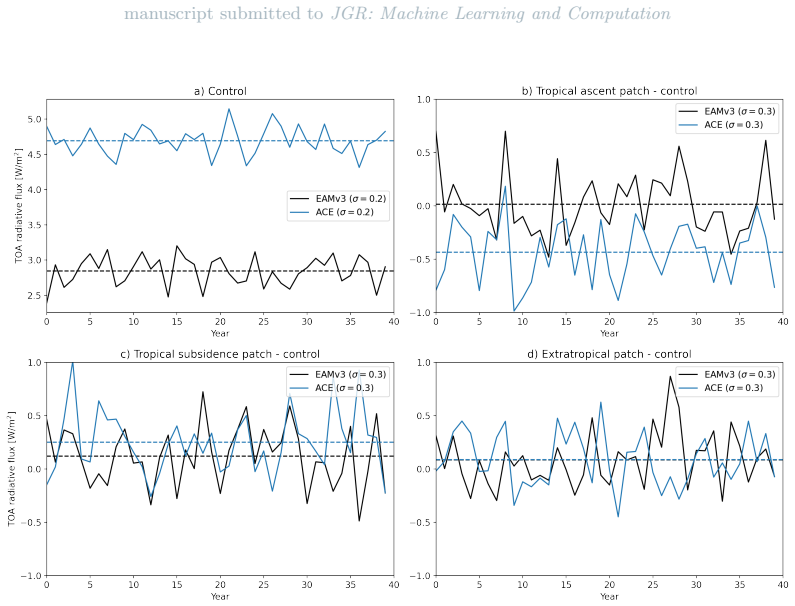
The load-bearing machinery is the combination of the emulator itself and the Green's-function construction. ACE2 is an autoregressive machine-learning climate emulator at 1-degree horizontal resolution and 6-hourly time steps, trained with a two-step loss, a 384-dimensional embedding, and global dry-air and moisture conservation, so it learns the radiative response implicitly rather than by predicting clouds. The Green's-function construction follows the standard protocol: 109 ocean patches, each perturbed by a smooth cosine-squared SST anomaly reaching +2 K or -2 K at its center, with the response defined as the change in global-mean net TOA radiation normalized by the area-averaged SST anomaly, $(dN/dSST)_p = \Delta N_p / \langle \Delta SST_p \rangle$, and with an uncertainty estimate based on the interannual standard deviation $\sigma_N = 0.2$ W/m² and the 10-year patch and 20-year control lengths. The paper also uses the patch basis to reconstruct historical $\Delta N$ by superposing patch responses weighted by the SST anomaly at each patch center, which serves as the consistency check.
What would settle it
Extend the EAMv3 control and patch runs to 40 years for all 109 patch locations and estimate each patch's interannual standard deviation and autocorrelation; if any patch shows variability clearly above 0.2 W/m² or significant correlation between years, the 2-sigma thresholds marking the ACE–EAMv3 differences as significant, especially in the northeast Pacific, would need to be recomputed.
Extended reading notes
Core claim
The paper's central claim is that an autoregressive machine-learning emulator, ACE2, trained only on a 51-year historical SST-forced simulation of the EAMv3 global atmosphere model, can serve as a surrogate for EAMv3 in the standardized SST-patch experiments used to construct Green's functions. The emulator matches the spatial pattern of top-of-atmosphere radiative response for individual +2 K SST patches, reproduces the qualitative geography of the global mean radiation sensitivity to patch location (area-weighted spatial correlation 0.53 against the reference), and reconstructs the historical global-mean net TOA radiation anomaly over 1970–2020 about as well as the physics-based model's own Green's functions. The match is not exact: for a number of low-latitude patches, especially in the subtropical northeast Pacific, the difference between emulator and model sensitivity exceeds the estimated 2-sigma significance threshold of about 8 W/m²/K. The paper attributes the residual bias to insufficient diversity in the SST anomaly patterns sampled during training, and it reports that the emulator runs the whole suite about 100 times faster in wall-clock time.
Load-bearing premise
The significance claims assume that global-mean net TOA radiation has the same year-to-year variability (about 0.2 W/m²) and no serial correlation for every SST patch and the control run, although that value was verified for only the control and three representative patches.
Editorial extensions
If this is right
- The full 218-patch SST experiment suite runs in 2.3 wall-clock days on one GPU, versus 331 wall-clock days for EAMv3 on eight CPU nodes, a speedup of roughly 100 times.
- Because the emulator is cheap, every patch simulation can be extended to 40 years, which reduces the internal-variability noise floor for the sensitivity maps by about a factor of two.
- The ACE and EAMv3 radiative-sensitivity maps have an area-weighted spatial pattern correlation of 0.53, and ACE is biased relative to EAMv3 at many low-latitude patches, most strongly in the 0–20°N eastern Pacific.
- Green's functions from both models reproduce the historical global annual-mean net TOA radiation anomaly, with the ACE reconstruction showing reduced interannual variability ($\sigma = 0.32$ W/m²) relative to its 0.50 W/m² target.
- The paper concludes that the current emulator is not yet a substitute for physics-model Green's functions, framing the result as a feasibility demonstration and a target for further training improvements.
Reading between the lines
- If the paper's training-diversity hypothesis is correct, the northeast Pacific bias is a data limitation rather than an architectural one; retraining on a long pre-industrial control run or on a subset of the patch simulations themselves should shrink it, and the emulator's low cost makes that test cheap.
- Holding the patch protocol fixed and comparing ACE2 trained on EAMv3 with the same emulator trained on reanalysis would separate errors introduced by the reference training data from errors intrinsic to the emulator, something the paper's comparison with earlier reanalysis-trained versions only hints at.
- The emulator reproduces cloud-driven radiative responses without predicting clouds, suggesting that the statistical relationship between resolved atmospheric state and radiation is learnable directly; if so, the same strategy could be applied to other subgrid processes too expensive to simulate explicitly.
- Using an ensemble of ACE2 random seeds rather than a single checkpoint for the patch runs could reduce emulator-specific internal variability and sharpen the significance map at negligible additional cost.
Signed reviews
Editorial analysis
A structured set of objections, weighed in public.
Referee Report
Summary. The paper trains the ACE2 machine-learning emulator on a 51-year (1970-2020) AMIP-style EAMv3 simulation and then applies the GFMIP Green's function protocol to compare ACE with the EAMv3 reference model. The authors run 109 warm and 109 cold SST patch simulations plus a control for both ACE and EAMv3, extending the ACE runs to 40 years while using the GFMIP-standard 10-year patches for the main comparisons. They find that the spatial patterns of TOA radiative response to individual SST patches are qualitatively similar between ACE and EAMv3, that the derived global-mean TOA radiative sensitivity maps are broadly consistent but show statistically significant discrepancies for some patches, particularly in the subtropical northeast Pacific, and that Green's function reconstructions of the historical 1970-2020 TOA radiation time series are reasonable for both models. They also report that ACE completes the GFMIP suite roughly 100 times faster in wall-clock time than EAMv3 under the configurations used.
Significance. If the results hold, the paper provides a valuable demonstration that a learned atmospheric emulator can approximate the patterned-SST Green's functions of a full-physics climate model at a fraction of the computational cost, which could make pattern-effect diagnostics accessible for many more experiments and models. The study is carefully designed: the GFMIP protocol is followed closely, the ACE patch simulations are genuine out-of-sample tests, the EAMv3 reference patch simulations provide a non-circular ground truth for the head-to-head comparison, and the authors report uncertainty estimates and explicitly acknowledge the limits of their training data. The open release of training/evaluation code, experiment scripts, and the ACE2-EAMv3 checkpoint is a strength that supports reproducibility. The main caveat is that the statistical significance of the ACE-EAMv3 discrepancies rests on an extrapolated interannual-variability assumption; if that assumption is too optimistic, some headline discrepancies, especially in the northeast Pacific, may not be significant.
major comments (1)
- [Section 3.3, Eqs. (3)-(7)] The issue is directly testable with the available ACE data and a small number of targeted EAMv3 runs, so it is fixable within the manuscript's scope.
minor comments (5)
- [Abstract and Section 2.1] The 'approximately 100 times faster' claim in the Abstract refers to the wall-clock time for running the GFMIP suite after training, but the training cost (50 epochs at 1.7 hours per epoch on 16 A100 GPUs) is substantial; the text should explicitly state that the training cost is excluded, or provide an end-to-end comparison including training.
- [Section 3.3] The description of the 'average' method as 'the average of the one-sided warm and cold-patch results' is inconsistent with the formula in Eq. (5), which corresponds to the warm-minus-cold difference divided by two; please reword to avoid confusion.
- [Section 3.4 and Figure 7] The reconstruction comparison uses 40-year ACE patch simulations but 10-year EAMv3 patch simulations; this difference in averaging length should be discussed when interpreting the reported standard deviations and RMSE values, since it affects the noise level in the reconstructed Green's functions.
- [Figure 7 caption] The sentence 'The RMSE for Green's functions ACE with respect to EAMv3 historical target is 0.43' is ambiguous; please clarify whether this is an additional cross-target metric and also report the RMSE of the ACE reconstruction against its own target.
- [Figures 5 and 6] The text refers to 'darkened regions' while the figure captions refer to 'hatches' to indicate significance; please make the terminology consistent.
Circularity Check
No significant circularity: the central ACE-vs-EAMv3 GFMIP comparison is an out-of-sample benchmark, and the historical reconstruction is explicitly labeled a consistency check.
full rationale
The central comparison is not circular. ACE2 is trained on the EAMv3 AMIP simulation, while the GFMIP patch experiments are held out: the paper states, 'Since ACE2-EAMv3 is trained on the AMIP-style EAMv3 reference simulation, all patch simulations are out-of-sample tests of the emulator.' The EAMv3 reference patch simulations used for the sensitivity maps and for the significance test of ACE-vs-EAMv3 differences were run independently under the GFMIP protocol and were not used to fit or select ACE, so the headline discrepancy claim is a genuine benchmark rather than a fitted input. The historical reconstruction is explicitly introduced as a self-consistency check ('A consistency check that helps confirm their credibility') and is not presented as an independent prediction; it uses the same model's own target, which is a stated limitation rather than a disguised input. The selection of the checkpoint and random seed by inline-inference RMSE on the AMIP period is a model-selection step and could make the emulator's historical biases look somewhat favorable, but it does not enter the GFMIP patch-response equations (Eqs. 2, 3, 5, 7) by construction, so it is not a circular reduction. Likewise, the uniform sigma_N = 0.2 W/m^2 assumption is an empirical extrapolation and a legitimate uncertainty concern, but it is not circular: the significance thresholds are derived from an explicit statistical model applied to an independently estimated variability, not from the discrepancy being tested. Self-citations to ACE2 training and GFMIP protocol are normal methodological references and are not load-bearing substitutes for the independent EAMv3 benchmark.
Assumptions & free parameters
free parameters (3)
- ACE random seed / checkpoint selection =
seed with lowest 1970-2020 net TOA radiation RMSE
- Patch valid-grid-point threshold =
3% of patch grid points
- Interannual standard deviation sigma_N =
0.2 W/m2
assumptions (4)
- domain assumption GFMIP SST patch response is sufficiently linear that warm and cold patch results can be averaged and superposed (BJ24 Eqns. 2-3, this paper Eqns. 8-9).
- domain assumption TOA global-mean net radiation interannual variability is uncorrelated year-to-year and uniform across patch locations with sigma_N = 0.2 W/m2.
- standard math The GFMIP patch grid (centers every 10 degrees latitude and 40 degrees longitude, Eq. 1) forms a basis adequate to reconstruct historical SST anomalies for TOA radiation reconstructions.
- domain assumption The 51-year EAMv3 AMIP simulation is a representative sample of EAMv3 behavior for the out-of-sample GFMIP SST perturbations.
Cite this review
Pith. "Pith review of Applying the ACE2 Emulator to SST Green's Functions for the E3SMv3 Global Atmosphere Model." pith.science (2026). https://pith.science/paper/MGWBXLZB
@misc{pith2026250508742,
  author       = {Pith},
  title        = {Pith review of: Applying the ACE2 Emulator to SST Green's Functions for the E3SMv3 Global Atmosphere Model},
  year         = {2026},
  howpublished = {\url{https://pith.science/paper/MGWBXLZB}},
  note         = {Machine review of arXiv:2505.08742}
}
read the original abstract
Green's functions are a useful technique for interpreting atmospheric state responses to changes in the spatial pattern of sea surface temperature (SST). Here we train version 2 of the Ai2 Climate Emulator (ACE2) on reference historical SST simulations of the US Department of Energy's EAMv3 global atmosphere model. We compare how well the SST Green's functions generated by ACE2 match those of EAMv3, following the protocol of the Green's Function Model Intercomparison Project (GFMIP). The spatial patterns of top-of-atmosphere (TOA) radiative response from the individual GFMIP SST patch simulations are similar for ACE and the EAMv3 reference. The derived sensitivity of global net TOA radiation sensitivity to SST patch location is qualitatively similar in ACE as in EAMv3, but there are statistically significant discrepancies for some SST patches, especially over the subtropical northeast Pacific. These discrepancies may reflect insufficient diversity in the SST patterns sampled over the course of the EAMv3 AMIP simulation used for training ACE. Both ACE and EAMv3 Green's functions reconstruct the historical record of the global annual-mean TOA radiative flux from a reference EAMv3 AMIP simulation reasonably well. Notably, under our configuration and compute resources, ACE achieves these results approximately 100 times faster in wall-clock time compared to EAMv3, highlighting its potential as a powerful and efficient tool for tackling other computationally intensive problems in climate science.
Figures


Figures from the paper (4 more)


Reference graph
Works this paper leans on
-
[1]
alessi_surface_2023 APACrefauthors Alessi, M J. \ Rugenstein, M A A. APACrefauthors \ 2023 . Surface Temperature Pattern Scenarios Suggest Higher Warming Rates Than Current Projections Surface Temperature Pattern Scenarios Suggest Higher Warming Rates Than Current Projections . Geophysical Research Letters 50 23 e2023GL105795 . APACrefDOI doi:10.1029/2023...
-
[2]
barsugli_global_2002 APACrefauthors Barsugli, J J. \ Sardeshmukh, P D. APACrefauthors \ 2002 . Global Atmospheric Sensitivity to Tropical SST Anomalies throughout the Indo - Pacific Basin Global Atmospheric Sensitivity to Tropical SST Anomalies throughout the Indo - Pacific Basin . Journal of Climate
work page 2002
-
[3]
bloch-johnson_greens_2024 APACrefauthors Bloch-Johnson, J. , Rugenstein, M A A. , Alessi, M J. , Proistosescu, C. , Zhao, M. , Zhang, B. Zhou, C. APACrefauthors \ 2024 . The Green 's Function Model Intercomparison Project ( GFMIP ) Protocol The Green 's Function Model Intercomparison Project ( GFMIP ) Protocol . Journal of Advances in Modeling Earth Syste...
-
[4]
branstator_analysis_1985 APACrefauthors Branstator, G. APACrefauthors \ 1985 . Analysis of General Circulation Model Sea - Surface Temperature Anomaly Simulations Using a Linear Model . Part I : Forced Solutions Analysis of General Circulation Model Sea - Surface Temperature Anomaly Simulations Using a Linear Model . Part I : Forced Solutions . Journal of...
work page 1985
-
[5]
clark_ace2-som_2024 APACrefauthors Clark, S K. , Watt-Meyer, O. , Kwa, A. , McGibbon, J. , Henn, B. , Perkins, W A. Bretherton, C S. APACrefauthors \ 2024 . ACE2 - SOM : Coupling an ML atmospheric emulator to a slab ocean and learning the sensitivity of climate to changed CO2. ACE2 - SOM : Coupling an ML atmospheric emulator to a slab ocean and learning t...
-
[6]
, Proistosescu, C
dong_attributing_2019 APACrefauthors Dong, Y. , Proistosescu, C. , Armour, K C. \ Battisti, D S. APACrefauthors \ 2019 . Attributing Historical and Future Evolution of Radiative Feedbacks to Regional Warming Patterns using a Green ’s Function Approach : The Preeminence of the Western Pacific Attributing Historical and Future Evolution of Radiative Feedbac...
2019
-
[7]
Duncan2024 APACrefauthors Duncan, J P C. , Wu, E. , Golaz, J. , Caldwell, P M. , Watt‐Meyer, O. , Clark, S K. Bretherton, C S. APACrefauthors \ 2024 . Application of the AI2 Climate Emulator to E3SMv2’s Global Atmosphere Model, With a Focus on Precipitation Fidelity Application of the ai2 climate emulator to e3smv2’s global atmosphere model, with a focus ...
-
[8]
Eyring2016 APACrefauthors Eyring, V. , Bony, S. , Meehl, G A. , Senior, C A. , Stevens, B. , Stouffer, R J. \ Taylor, K E. APACrefauthors \ 2016 . Overview of the Coupled Model Intercomparison Project Phase 6 (CMIP6) experimental design and organization Overview of the coupled model intercomparison project phase 6 (cmip6) experimental design and organizat...
Show all 15 references
-
[9]
, Boyle, J S
gates_overview_1999 APACrefauthors Gates, W L. , Boyle, J S. , Covey, C. , Dease, C G. , Doutriaux, C M. , Drach, R S. Williams, D N. APACrefauthors \ 1999 . An Overview of the Results of the Atmospheric Model Intercomparison Project ( AMIP I ) An Overview of the Results of th...
1999
-
[10]
, Rugenstein, M
loon_reanalysis-based_2025 APACrefauthors Loon, S V. , Rugenstein, M. \ Barnes, E A. APACrefauthors \ 2025 . Reanalysis-based Global Radiative Response to Sea Surface Temperature Patterns : Evaluating the Ai2 Climate Emulator . Reanalysis-based Global Radiative Response to Sea...
-
[11]
, Dresdner, G
WattMeyer2023 APACrefauthors Watt-Meyer, O. , Dresdner, G. , McGibbon, J. , Clark, S K. , Henn, B. , Duncan, J. Bretherton, C S. APACrefauthors \ 2023 . ACE: A fast, skillful learned global atmospheric model for climate prediction. ACE: A fast, skillful learned global atmosphe...
-
[12]
, Henn, B
watt-meyer_ace2_2024 APACrefauthors Watt-Meyer, O. , Henn, B. , McGibbon, J. , Clark, S K. , Kwa, A. , Perkins, W A. Bretherton, C S. APACrefauthors \ 2024 . ACE2 : Accurately learning subseasonal to decadal atmospheric variability and forced responses. ACE2 : Accurately learn...
-
[13]
, Terai, C R
xie2025energy APACrefauthors Xie, S. , Terai, C R. , Wang, H. , Tang, Q. , Fan, J. , Burrows, S M. others APACrefauthors \ 2025 . The Energy Exascale Earth System Model Version 3. Part I: Overview of the Atmospheric Component The energy exascale earth system model version 3. p...
2025
-
[14]
, Zhao, M
zhang_using_2023 APACrefauthors Zhang, B. , Zhao, M. \ Tan, Z. APACrefauthors \ 2023 . Using a Green ’s Function Approach to Diagnose the Pattern Effect in GFDL AM4 and CM4 Using a Green ’s Function Approach to Diagnose the Pattern Effect in GFDL AM4 and CM4 . Journal of Clima...
2023 doi
-
[15]
, Zelinka, M D
zhou_analyzing_2017 APACrefauthors Zhou, C. , Zelinka, M D. \ Klein, S A. APACrefauthors \ 2017 . Analyzing the dependence of global cloud feedback on the spatial pattern of sea surface temperature change with a Green 's function approach Analyzing the dependence of global clo...
2017 doi
Reviewed August 15, 2026 · model on record in the stance chip above.
Discussion (0). Continue with ORCID to comment.