REVIEW 4 major objections 6 minor 1 cited by
Opening the Black Box of Local Projections
T0 review · 4 major / 6 minor · reviewed 2026-08-15 · deepseek-v4-flash
Pith's one-line read This paper shows that every local projection estimate decomposes into weighted contributions from individual historical episodes, with weights interpretable as purified shocks or proximity scores.
desk verdict A useful and mostly sound diagnostic framework for local projections, but the headline claims about dominant historical episodes need uncertainty quantification before they can be taken at face value. read the letter →
The pith
A machine-rendered reading of the paper's core claim, the machinery that carries it, and where it could break.
The reading
What carries the argument
The central object is the weight vector $w = [(X'X)^{-1}X']_{2,:}$, the row of the OLS projection matrix that selects the shock coefficient. The Frisch-Waugh-Lovell theorem turns this into $w_t = s_t^*/T$, giving the weights a purified-shock meaning. The dual solution of least squares turns it into a proximity score: in the whitened feature space $F_t = X_t U \Lambda^{-1/2}$, each $w_t$ is the inner product $\langle F^\delta_\tau - F^0_\tau, F_t\rangle$, so the coefficient is a similarity-weighted average of past outcomes. In Random Forests, weights are recovered by averaging, across trees, the indicator that observation $t$ falls in the same leaf as the hypothetical intervention; the nonlinear impulse response is the difference between two such weight vectors, one for shock $\delta$ and one for no shock.
What would settle it
For each of the four applications, remove the single highest-contribution episode identified by the decomposition: World War II for the recession fiscal multiplier, the 1964 Mount Agung shock for climate, the 1976-1978 loosening sequence and Nixon episodes for monetary policy, and the 2007-2008 financial distress cluster for financial shocks, then re-estimate; the paper's central concentration claim predicts each estimate should largely collapse, and verifying this uniformly would settle how much of each result depends on one event.
Extended reading notes
Core claim
This paper's central claim is that any local projection coefficient is a weighted sum of historical outcomes: $\hat{\beta}_h = \sum_{t=1}^{T} w_t y_{t+h}$, where $w$ is the second row of $(X'X)^{-1}X'$ and $y_{t+h}$ is the outcome realized $h$ periods after observation $t$. The paper then gives the weights two interpretations. By the Frisch-Waugh-Lovell theorem, $w_t = s_t^*/T$, where $s_t^*$ is the shock $s_t$ residualized on the controls and standardized, so each contribution is a purified shock times the realized outcome. Through the dual form of least squares, $w_t$ is instead the difference between the inner products of a hypothetical intervention and each historical intervention in an orthonormal feature space, which makes OLS an estimator that upweights past episodes resembling the intervention being studied. Because Random Forest predictions and many other machine-learning predictors are linear combinations of the outcome, the same decomposition carries over to nonlinear local projections, where weights differ by horizon, shock sign, and context.
Load-bearing premise
The narrative reading of the decomposition, that specific episodes like Nixon's pressure or World War II are what drive an estimate, presupposes the standard local projection assumptions of exogenous shocks, correctly specified controls, and stable coefficients; if those fail, the weights still decompose the OLS number mechanically, but the historical attribution is not identified.
Editorial extensions
If this is right
- Each LP estimate can be plotted as an evidence curve, with cumulative contributions over time showing whether support is broad or concentrated in one episode.
- The concentration statistics $WC$ and $CC$, which report the share of absolute weights and contributions held by the top 10% of observations, give a one-number diagnostic for external validity.
- The framework explains the monetary price puzzle as misattribution of 1970s stagflation to tightening, and shows that narrative monetary shocks identify effects almost entirely from politically motivated loosening in the 1970s.
- State-dependent fiscal multipliers estimated from military spending shocks are almost entirely driven by World War II, and long-run climate damage estimates are heavily influenced by the 1964 Mount Agung eruption paired with the post-war boom, making those long-run results fragile.
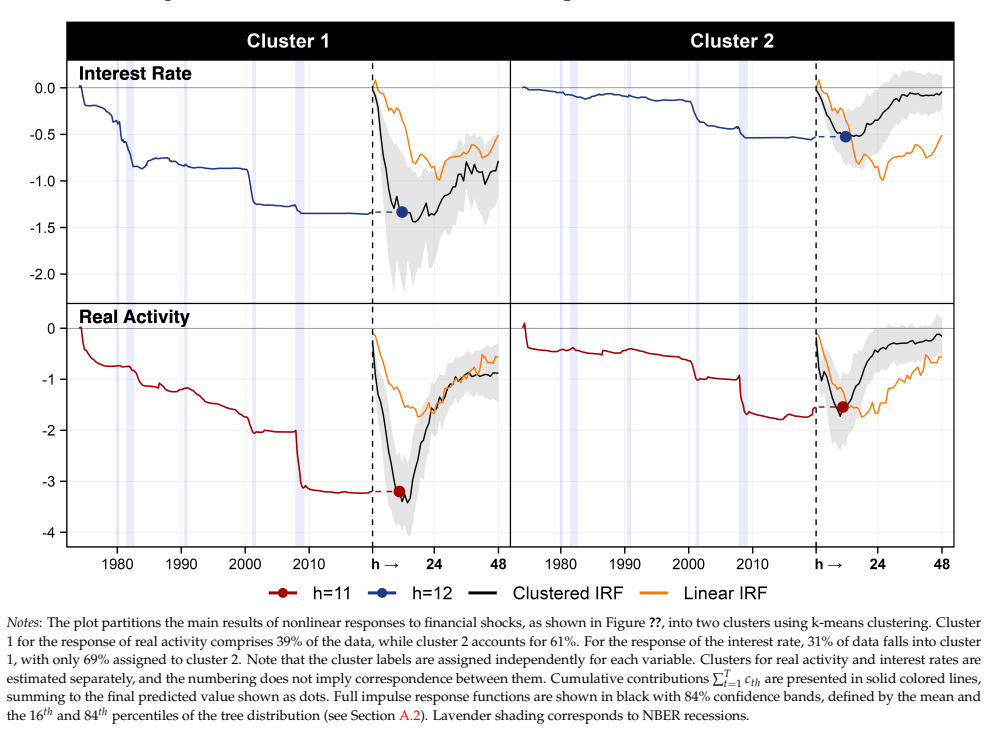
- Nonlinear Random Forest local projections can be read with the same tools, revealing that contractionary narrative monetary shocks yield null effects while expansionary effects are concentrated in identifiable episodes such as Nixon's pressure on the Federal Reserve.
Reading between the lines
- A natural extension would make the decomposition a pre-registered robustness check: report $WC$, $CC$, and the dominant episode for every LP estimate, and treat estimates whose top episode accounts for most of the coefficient with caution.
- The same machinery could be applied to panel local projections to separate time-period from cross-sectional contributions, and to two-stage least squares by decomposing the first and second stages separately.
- If concentration is as high as the applications suggest, then nonlinear and state-dependent effects estimated from the same short samples inherit the same fragility; the paper's trimming exercises indicate that removing one episode often collapses the estimate, a test that could be standardized for all four applications.
- Because the decomposition is mechanical, it does not by itself validate the causal reading; it equips a substantive identification argument with a precise picture of where the evidence lives.
Signed reviews
Editorial analysis
A structured set of objections, weighed in public.
Referee Report
Summary. This paper introduces a decomposition of local projection (LP) estimates of impulse responses into a sum over time of contributions c_th = w_t y_{t+h}, where w is the second row of (X'X)^{-1}X' (Eqs. 3-4). For OLS, the paper gives two interpretations of w: as standardized, purified shocks via the Frisch-Waugh-Lovell theorem (Eqs. 6-8), and as proximity scores between a hypothetical intervention and past interventions in an orthonormalized regressor space (Eqs. 9-15). The proximity interpretation is extended to random forest LPs by expressing predictions as weighted averages of outcomes. Two concentration statistics, WC and CC, quantify the share of top-Q% weights and contributions. The framework is applied to monetary, fiscal, climate, and financial shocks; the authors report that estimates are often concentrated in a small number of identifiable episodes such as Nixon-era monetary loosening, WWII, and the 1963 Mount Agung eruption.
Significance. If the empirical claims can be supported with inference, this is a useful and original diagnostic. The OLS decomposition is an exact, parameter-free identity, and the FWL interpretation is rigorous. The proximity interpretation provides an intuitive bridge to machine-learning LPs, and the RF weight recovery is clearly described. The paper ships R code and slides, and the fiscal and climate applications include transparent robustness checks that, if anything, undercut the headline episode attribution. The main value is a diagnostic that quantifies how many historical observations actually support an IRF, which is a real gap in the LP toolkit.
major comments (4)
- [Section 3; Tables 1-4] The headline concentration statistics (WC, CC) and the top-contribution episode rankings are reported as point estimates with no measure of sampling uncertainty. Because w is a nonlinear function of the full sample through (X'X)^{-1}, a single influential observation can change the top-contribution ranking, and the paper's own adversarial checks demonstrate exactly this fragility: trimming the top and bottom 1% of fiscal weights collapses both state-dependent IRFs to zero (Figure 6), and starting the climate sample in 1985 eliminates the long-run effect attributed to Mount Agung (Figure 9). Please add bootstrap or wild bootstrap confidence intervals, or subsample stability analyses, for WC, CC, and the identity of top contributors, and calibrate the claims in the Abstract and Section 4 to what survives that inference.
- [Section 3.1; footnote 2] The narrative attribution of contributions to events such as 'Nixon's interference with the Fed' or 'stagflation' is a causal reading of the decomposition; it inherits the identifying assumptions of the LP listed in footnote 2 (exogeneity, correct controls, coefficient stability). Footnote 2 correctly states that the decomposition itself is mechanical, but the Introduction and Abstract do not carry that caveat. Please either soften the episode-attribution language to descriptive weighting, or provide evidence that the attributions are stable under alternative control sets and placebo shock series with the same autocorrelation structure. A placebo exercise would be a concrete way to show that top contributions are not generated by a null shock process.
- [Appendix A.2.1; Section 3.1 nonlinear results] The random forest design forces shock variables into every split via always.split.variables, and the paper states that without this adjustment the shock series would be effectively ignored by the RF. The nonlinear findings, especially the null contractionary monetary response and the sparse proximity weights, may therefore be artifacts of this selective regularization. Sensitivity to min.node.size is reported, but sensitivity to mtry and to always.split.variables is not. Please report results for a grid of these tuning parameters, or a data-driven choice such as cross-validation, and show the corresponding weights and IRFs so the reader can assess how much of the nonlinear concentration is model-induced.
- [Section 2.2.2; Figures 2 and 14] The proximity interpretation of w in the correlated case uses the scenario vectors X^delta_tau and X^0_tau, but the empirical proximity plots do not state how Z_tau is chosen. Since beta_h is invariant to Z_tau in the linear model while w's decomposition into cosine and norm components in (12)-(15) is not, the 'proximity' narrative depends on an arbitrary choice of the scenario. Please specify the rule used for Z_tau in Figures 2 and 14 and check the sensitivity of the reported proximity patterns to alternative scenario definitions, such as the sample mean, the last observation, or an explicit policy counterfactual.
minor comments (6)
- [Eq. (3)] The notation dIRF with a hat is ambiguous; suggest writing the estimator as \widehat{IRF}_{s\to y}(h,1) = \hat\beta_h and defining w as a row vector consistently.
- [Eqs. (6)-(8)] Var(\tilde s_t) in (7) should be the sample variance of the residual series to be numerically exact; please state this explicitly.
- [Eq. (24)] The approximation w_t \hat\nu_{t+h} \approx IF_t is informal; define the approximation error and state that it holds exactly only under the i.i.d. cross-sectional conditions described in the text.
- [Table 1] The repeated quotation marks in Table 1 should be replaced with actual numbers or an explicit statement that WC is horizon-invariant for linear models.
- [Figure 23 caption] The caption refers to 'Figure ??'; the cross-reference should be fixed to Figure 10.
- [References] The in-text citation 'Zeev et al. (2023)' should be expanded to 'Ben Zeev, Ramey, and Zubairy (2023)' to match the reference list.
Circularity Check
No significant circularity: the LP decomposition is a mechanical identity and the proximity/FWL interpretations are derived within the paper.
full rationale
The paper's central object is an algebraic identity: beta-hat_h is written as the second row of (X'X)^{-1}X' times y_h (Eq. 3), and then as a sum of contributions c_th = w_t y_{t+h} (Eq. 4). This holds for any OLS local projection by the normal equations; no parameter is fitted to reproduce a target result. The FWL representation (Eqs. 6-8) expresses w as standardized residuals from projecting the shock on controls, which is a direct algebraic consequence. The proximity interpretation (Eqs. 9-15) is also derived in-paper using the dual OLS identity X'(X X')^+ and an eigen-transformation of the regressor space; it does not assume the interpretation it claims to establish. The citations to Goulet Coulombe (2025) and Goulet Coulombe et al. (2024) provide terminology and prior interpretative framing for predictions, but the coefficient-level extension is not imported: the relevant algebra appears in the manuscript. The empirical episode attributions are descriptive properties of the estimated weights and outcomes, and the paper's own trimming and subsample exercises expose fragility rather than assuming it. The identification caveats in footnote 2 are acknowledged limitations on causal reading, not circularity in the decomposition itself. No uniqueness theorem, ansatz, or fitted quantity is smuggled in via self-citation, and the Random Forest design choices are openly disclosed and do not force the reported null tightening effects.
Assumptions & free parameters
free parameters (5)
- RF min.node.size =
5
- RF mtry =
1/15 of predictors
- always.split.variables =
shock lags and target lags forced into candidate splits
- Number of clusters in k-means =
2 per application
- Concentration threshold Q =
10
assumptions (7)
- standard math OLS normal equations and Frisch-Waugh-Lovell theorem
- standard math Moore-Penrose pseudoinverse dual equivalence (X'X)^{-1}X' = X'(X X')^+
- standard math Representer theorem for RKHS and Random Forest predictions linear in outcomes
- domain assumption Exogeneity and correct specification of LP shock series
- domain assumption Stationarity of transformed data in applications
- domain assumption Choice of scenario vector Z_tau in the linear proximity representation does not affect final weights
- domain assumption Random Forest is a consistent estimator of the conditional expectation given the DGP
Cite this review
Pith. "Pith review of Opening the Black Box of Local Projections." pith.science (2026). https://pith.science/paper/MKJ5JFOI
@misc{pith2026250512422,
  author       = {Pith},
  title        = {Pith review of: Opening the Black Box of Local Projections},
  year         = {2026},
  howpublished = {\url{https://pith.science/paper/MKJ5JFOI}},
  note         = {Machine review of arXiv:2505.12422}
}
read the original abstract
Local projections (LPs) are widely used in empirical macroeconomics to estimate impulse responses to policy interventions. Yet, in many ways, they are black boxes. It is often unclear what mechanism or historical episodes drive a particular estimate. We introduce a new decomposition of LP estimates into the sum of contributions of historical events, which is the product, for each time stamp, of a weight and the realization of the response variable. In the least squares case, we show that these weights admit two interpretations. First, they represent purified and standardized shocks. Second, they serve as proximity scores between the projected policy intervention and past interventions in the sample. Notably, this second interpretation extends naturally to machine learning methods, many of which yield impulse responses that, while nonlinear in predictors, still aggregate past outcomes linearly via proximity-based weights. Applying this framework to shocks in monetary and fiscal policy, global temperature, and the excess bond premium, we find that easily identifiable events-such as Nixon's interference with the Fed, stagflation, World War II, and the Mount Agung volcanic eruption-emerge as dominant drivers of often heavily concentrated impulse response estimates.
Figures


Figures from the paper (4 more)


Forward citations
Cited by 1 Pith paper
-
Bandwidth-Free Inference for Recursive Nonlinear Impulse Response Functions
The paper provides first-order, bootstrap, and finite-simulation inference for recursive nonlinear impulse responses computed from empirical residual quantiles, without density estimation or quantile-smoothing bandwidths.
Reference graph
Works this paper leans on
-
[1]
D., Jorda, O., and Kuersteiner, G
Angrist, J. D., Jorda, O., and Kuersteiner, G. M. (2018). Semiparametric Estimates of Monetary Policy Effects : String Theory Revisited . Journal of Business & Economic Statistics , 36(3):371--387
2018
-
[2]
Angrist, J. D. and Krueger, A. B. (1999). Empirical strategies in labor economics. In Handbook of Labor Economics , volume 3, pages 1277--1366. Elsevier
1999
-
[3]
Aruoba, S. B. and Drechsel, T. (2024). Identifying monetary policy shocks: A natural language approach. Technical report, National Bureau of Economic Research
2024
-
[4]
Athey, S., Bayati, M., Imbens, G., and Qu, Z. (2019). Ensemble methods for causal effects in panel data settings. In AEA Papers and Proceedings , volume 109, pages 65--70. American Economic Association 2014 Broadway, Suite 305, Nashville, TN 37203
work page 2019
-
[5]
Auerbach, A. J. and Gorodnichenko, Y. (2012). Measuring the output responses to fiscal policy. American Economic Journal: Economic Policy , 4(2):1--27
work page 2012
-
[6]
Auerbach, A. J. and Gorodnichenko, Y. (2013). Fiscal multipliers in recession and expansion. In Alesina, A. and Giavazzi, F., editors, Fiscal Policy after the Financial Crisis , pages 63--98. University of Chicago Press
work page 2013
-
[7]
Bachmann, R. and Sims, E. R. (2012). Confidence and the transmission of government spending shocks. Journal of Monetary Economics , 59(3):235--249
work page 2012
-
[8]
Balke, N. S., Emery, K. M., et al. (1994). Understanding the price puzzle. Federal Reserve Bank of Dallas Economic Review, Fourth Quarter , pages 15--26
work page 1994
Show all 83 references
-
[9]
Barnichon, R., Matthes, C., and Ziegenbein, A. (2022). Are the effects of financial market disruptions big or small? Review of Economics and Statistics , 104(3):557--570
2022
-
[10]
and Mesters, G
Barnichon, R. and Mesters, G. (2025). Innovations meet narrative - improving the power-credibility trade-off in macro. Technical report
2025
-
[11]
Belkin, M., Hsu, D., Ma, S., and Mandal, S. (2019). Reconciling modern machine-learning practice and the classical bias--variance trade-off. Proceedings of the National Academy of Sciences , 116(32):15849--15854
2019
-
[12]
and Pappa, E
Ben Zeev, N. and Pappa, E. (2017). Chronicle of a war foretold: The macroeconomic effects of anticipated defence spending shocks. The Economic Journal , 127(603):1568--1597
2017
-
[13]
S., Boivin, J., and Eliasz, P
Bernanke, B. S., Boivin, J., and Eliasz, P. (2005). Measuring the effects of monetary policy: a factor-augmented vector autoregressive (favar) approach. The Quarterly Journal of Economics , 120(1):387--422
2005
-
[14]
S., Gertler, M., Watson, M., Sims, C
Bernanke, B. S., Gertler, M., Watson, M., Sims, C. A., and Friedman, B. M. (1997). Systematic monetary policy and the effects of oil price shocks. Brookings Papers on Economic Activity , 1997(1):91--157
1997
-
[15]
and K \"a nzig, D
Bilal, A. and K \"a nzig, D. R. (2024). The macroeconomic impact of climate change: Global vs. local temperature. Technical report, National Bureau of Economic Research
2024
-
[16]
G., Rapach, D., Sch \"u tte, E
Borup, D., Coulombe, P. G., Rapach, D., Sch \"u tte, E. C. M., and Schwenk-Nebbe, S. (2022). The anatomy of out-of-sample forecasting accuracy. FRB Atlanta Working Paper
2022
-
[17]
Breiman, L. (1996). Bagging predictors. Machine Learning , 24(2):123--140
1996
-
[18]
Breiman, L. (2001). Random forests. Machine Learning , 45(1):5--32
2001
-
[19]
J., and Olshen, R
Breiman, L., Friedman, J., Stone, C. J., and Olshen, R. A. (1984). Classification and regression trees . CRC press
1984
-
[20]
Brissimis, S. N. and Magginas, N. S. (2006). Forward-looking information in var models and the price puzzle. Journal of Monetary Economics , 53:1225--1234
2006
-
[21]
Brunnermeier, M. K. and Sannikov, Y. (2014). A macroeconomic model with a financial sector. American Economic Review , 104(2):379--421
2014
-
[22]
and Joseph, A
Buckmann, M. and Joseph, A. (2023). An interpretable machine learning workflow with an application to economic forecasting. International Journal of Central Banking , 19(4):449--552
2023
-
[23]
C., Dunn, A., Hood, K
Chen, J. C., Dunn, A., Hood, K. K., Driessen, A., and Batch, A. (2019). Off to the races: A comparison of machine learning and alternative data for predicting economic indicators. In Big Data for 21st Century Economic Statistics . University of Chicago Press
2019
-
[24]
Chernozhukov, V., Chetverikov, D., Demirer, M., Duflo, E., Hansen, C., Newey, W., and Robins, J. (2018). Double/debiased machine learning for treatment and structural parameters
2018
-
[25]
J., Eichenbaum, M., and Evans, C
Christiano, L. J., Eichenbaum, M., and Evans, C. L. (1996). The effects of monetary policy shocks: Evidence from the flow of funds. Review of Economics and Statistics , 78(1):16--34
1996
-
[26]
J., Eichenbaum, M., and Evans, C
Christiano, L. J., Eichenbaum, M., and Evans, C. L. (1999). Monetary policy shocks: What have we learned and to what end? In Handbook of Macroeconomics , volume 1, pages 65--148. Elsevier
1999
-
[27]
Cloyne, J., Jord \`a , \`O ., and Taylor, A. M. (2023). State-dependent local projections: Understanding impulse response heterogeneity. Technical report, National Bureau of Economic Research
2023
-
[28]
Cook, R. D. and Weisberg, S. (1980). Characterizations of an empirical influence function for detecting influential cases in regression. Technometrics , 22(4):495--508
1980
-
[29]
and MacKinnon, J
Davidson, R. and MacKinnon, J. G. (2004). Econometric theory and methods , volume 5. Oxford University Press New York
2004
-
[30]
F., and Olken, B
Dell, M., Jones, B. F., and Olken, B. A. (2012). Temperature shocks and economic growth: Evidence from the last half century. American Economic Journal: Macroeconomics , 4(3):66--95
2012
-
[31]
Drechsel, T. (2024). Estimating the effects of political pressure on the fed: a narrative approach with new data. Technical report, National Bureau of Economic Research
2024
-
[32]
and Renault, E
Dufour, J.-M. and Renault, E. (1998). Short Run and Long Run Causality in Time Series : Theory . Econometrica , 66(5)
1998
-
[33]
A., editor (2005)
Epstein, G. A., editor (2005). Financialization and the World Economy . Edward Elgar Publishing
2005
-
[34]
H., Liang, T., and Misra, S
Farrell, M. H., Liang, T., and Misra, S. (2020). Deep learning for individual heterogeneity: An automatic inference framework. arXiv preprint arXiv:2010.14694
2020 arXiv
-
[35]
M., and Lemieux, T
Firpo, S., Fortin, N. M., and Lemieux, T. (2009). Unconditional quantile regressions. Econometrica , 77(3):953--973
2009
-
[36]
Forni, M., Gambetti, L., Maffei-Faccioli, N., and Sala, L. (2024). Nonlinear transmission of financial shocks: Some new evidence. Journal of Money, Credit and Banking , 56(1):5--33
2024
-
[37]
and Zou, J
Ghorbani, A. and Zou, J. (2019). Data shapley: Equitable valuation of data for machine learning. In International Conference on Machine Learning , pages 2242--2251. PMLR
2019
-
[38]
D., Deshpande, S., and Broderick, T
Ghosh, S., Stephenson, W., Nguyen, T. D., Deshpande, S., and Broderick, T. (2020). Approximate cross-validation for structured models. Advances in Neural Information Processing Systems , 33:8741--8752
2020
-
[39]
and Zakraj s ek, E
Gilchrist, S. and Zakraj s ek, E. (2012). Credit spreads and business cycle fluctuations. American Economic Review , 102(4):1692--1720
2012
-
[40]
M., Kilian, L., and Pesavento, E
Gon c alves, S., Herrera, A. M., Kilian, L., and Pesavento, E. (2024). State-dependent local projections. Journal of Econometrics , page 105702
2024
-
[41]
M., , Kilian, L., and Pesavento, E
Gonçalves, S., Herrera, A. M., , Kilian, L., and Pesavento, E. (2024). Nonparametric Local Projections . Federal Reserve Bank of Dallas, Working Papers , 2024(2414)
2024
-
[42]
and Lee, B
Gorodnichenko, Y. and Lee, B. (2020). Forecast Error Variance Decompositions with Local Projections . Journal of Business & Economic Statistics , 38(4):921--933
2020
-
[43]
Goulet Coulombe, P. (2020). Time-varying parameters as ridge regressions. arXiv preprint arXiv:2009.00401
2020 arXiv
-
[44]
Goulet Coulombe, P. (2024a). The macroeconomy as a random forest. Journal of Applied Econometrics , 39:401--421
2024
-
[45]
Goulet Coulombe, P. (2024b). To bag is to prune. Studies in Nonlinear Dynamics & Econometrics , (forthcoming)
2024
-
[46]
Goulet Coulombe, P. (2025). Ordinary least squares as an attention mechanism. Available at SSRN 5200864
2025
-
[47]
Goulet Coulombe, P., G \"o bel, M., and Klieber, K. (2024). Dual interpretation of machine learning forecasts. Available at SSRN 5029492
2024
-
[48]
Goulet Coulombe, P., Leroux, M., Stevanovic, D., and Surprenant, S. (2022). How is machine learning useful for macroeconomic forecasting? Journal of Applied Econometrics , 37(5):920--964
2022
-
[49]
Goulet Coulombe, P., Rapach, D., Sch \"u tte, E. C. M., and Schwenk-Nebbe, S. (2023). The anatomy of machine learning-based portfolio performance. Available at SSRN 4628462
2023
-
[50]
Hampel, F. R. (1974). The influence curve and its role in robust estimation. Journal of the American Statistical Association , 69(346):383--393
1974
-
[51]
Hanson, M. S. (2004). The ‘‘price puzzle’’ reconsidered. Journal of Monetary Economics , 51(6):1385--1413
2004
-
[52]
Hauzenberger, N., Huber, F., Klieber, K., and Marcellino, M. (2025). Machine learning the macroeconomic effects of financial shocks. Economics Letters , (forthcoming)
2025
-
[53]
Herbst, E. P. and Johannsen, B. K. (2024). Bias in local projections. Journal of Econometrics , 240(1):105655
2024
-
[54]
Huber, F., Matthes, C., and Pfarrhofer, M. (2024). General seemingly unrelated local projections. arXiv preprint arXiv:2410.17105
2024 arXiv
-
[55]
and Newey, W
Ichimura, H. and Newey, W. K. (2022). The influence function of semiparametric estimators. Quantitative Economics , 13(1):29--61
2022
-
[56]
and Taylor, A
Jord \`a , \`O . and Taylor, A. M. (2024). Local projections . National Bureau of Economic Research
2024
-
[57]
and Kim, Y
Kilian, L. and Kim, Y. J. (2011). How reliable are local projection estimators of impulse responses? Review of Economics and Statistics , 93(4):1460--1466
2011
-
[58]
and Wahba, G
Kimeldorf, G. and Wahba, G. (1971). Some results on tchebycheffian spline functions. Journal of Mathematical Analysis and Applications , 33(1):82--95
1971
-
[59]
and Plagborg-M ller, M
Koles \'a r, M. and Plagborg-M ller, M. (2024). Dynamic causal effects in a nonlinear world: the good, the bad, and the ugly. arXiv preprint arXiv:2411.10415
2024
-
[60]
Krippner, G. R. (2005). The financialization of the american economy. Socio-Economic Review , 3(2):173--208
2005
-
[61]
Kunsch, H. (1984). Infinitesimal robustness for autoregressive processes. The Annals of Statistics , pages 843--863
1984
-
[62]
Li, D., Plagborg-M ller, M., and Wolf, C. K. (2024). Local projections vs. vars: Lessons from thousands of dgps. Journal of Econometrics , 244(2):105722
2024
-
[63]
and Jeon, Y
Lin, Y. and Jeon, Y. (2006). Random forests and adaptive nearest neighbors. Journal of the American Statistical Association , 101(474):578--590
2006
-
[64]
McCracken, M. W. and Ng, S. (2016). Fred-md: A monthly database for macroeconomic research. Journal of Business & Economic Statistics , 34(4):574--589
2016
-
[65]
C., Vasconcelos, G
Medeiros, M. C., Vasconcelos, G. F., Veiga, \'A ., and Zilberman, E. (2021). Forecasting inflation in a data-rich environment: the benefits of machine learning methods. Journal of Business & Economic Statistics , 39(1):98--119
2021
-
[66]
Montiel Olea, J. L. and Plagborg-Møller, M. (2021). Local Projection Inference Is Simpler and More Robust Than You Think . Econometrica , 89(4):1789--1823
2021
-
[67]
and Piffer, M
Mumtaz, H. and Piffer, M. (2022). Impulse response estimation via flexible local projections. Available at SSRN 4088760
2022
-
[68]
and Steinsson, J
Nakamura, E. and Steinsson, J. (2018a). High-frequency identification of monetary non-neutrality: the information effect. The Quarterly Journal of Economics , 133(3):1283--1330
2018
-
[69]
and Steinsson, J
Nakamura, E. and Steinsson, J. (2018b). Identification in macroeconomics. Journal of Economic Perspectives , 32(3):59--86
2018
-
[70]
Newey, W. K. and McFadden, D. (1994). Large sample estimation and hypothesis testing. Handbook of Econometrics , 4:2111--2245
1994
-
[71]
Newey, W. K. and West, K. D. (1987). A simple, positive semi-definite, heteroskedasticity and autocorrelation consistent covariance matrix. Econometrica , 55(3):703--708
1987
-
[72]
Nordhaus, W. D. (1992). An optimal transition path for controlling greenhouse gases. Science , 258(5086):1315--1319
1992
-
[73]
Paranhos, L. (2024). How do firms’ financial conditions influence the transmission of monetary policy? A non-parametric local projection approach. Journal of Econometrics , page 105886
2024
-
[74]
Paul, P. (2020). The Time - Varying Effect of Monetary Policy on Asset Prices . The Review of Economics and Statistics , 102(4):690--704
2020
-
[75]
and Wolf, C
Plagborg-M ller, M. and Wolf, C. K. (2021). Local projections and vars estimate the same impulse responses. Econometrica , 89(2):955--980
2021
-
[76]
Ramey, V. A. (2011). Identifying government spending shocks: It's all in the timing. The Quarterly Journal of Economics , 126(1):1--50
2011
-
[77]
Ramey, V. A. and Zubairy, S. (2018). Government spending multipliers in good times and in bad: evidence from us historical data. Journal of Political Economy , 126(2):850--901
2018
-
[78]
Romer, C. D. and Romer, D. H. (2004). A new measure of monetary shocks: Derivation and implications. American Economic Review , 94(4):1055--1084
2004
-
[79]
Sch \"o lkopf, B., Herbrich, R., and Smola, A. J. (2001). A Generalized Representer Theorem . In International Conference on Computational Learning Theory , pages 416--426. Springer
2001
-
[80]
and Goyal, A
Welch, I. and Goyal, A. (2007). A Comprehensive Look at The Empirical Performance of Equity Premium Prediction . The Review of Financial Studies , 21(4):1455--1508
2007
-
[81]
Yitzhaki, S. (1996). On using linear regressions in welfare economics. Journal of Business & Economic Statistics , 14(4):478--486
1996
-
[82]
B., Ramey, V
Zeev, N. B., Ramey, V. A., and Zubairy, S. (2023). Do government spending multipliers depend on the sign of the shock? AEA Papers and Proceedings , 113:382--387
2023
-
[83]
Zhang, Y., Shen, J., Xiong, X., and Kwon, Y. (2024). Timeinf: Time series data contribution via influence functions. arXiv preprint arXiv:2407.15247
2024 arXiv
Reviewed August 15, 2026 · model on record in the stance chip above.
Discussion (0). Continue with ORCID to comment.