REVIEW 4 major objections 5 minor 54 references
Pulsar Cyclic Spectroscopy in the Partial-Deconvolution Regime: Benefits & Limitations
T0 review · 4 major / 5 minor · reviewed 2026-08-15 · deepseek-v4-flash
Pith's one-line read Cyclic spectroscopy remains useful when full deconvolution is impossible: partial phase retrieval still recovers the scintillation pattern and enables scattering-delay measurements.
desk verdict Worth engaging: the empirical partial-deconvolution demonstration is useful, but cyclic merit 2.0 is a calibrated fit rather than an independent predictor, and the phase-retrieval claim needs simulation support before it is trusted. read the letter →
The pith
A machine-rendered reading of the paper's core claim, the machinery that carries it, and where it could break.
The reading
What carries the argument
The load-bearing object is the cyclic spectrum $S_E(\nu,\alpha_k)=\langle E(\nu+\alpha_k/2)E^*(\nu-\alpha_k/2)\rangle$, through which the periodic pulsar signal is resampled at harmonics $\alpha_k=k/P$ of the pulse period, bypassing the usual time-frequency (Gabor) resolution limit. In the interstellar-medium case the cyclic spectrum factors into the intrinsic pulse transform times a bilinear product of the transfer function $H$, so the transfer function, and hence the dynamic wavefield $H(\nu,t)$, can be recovered by iterative deconvolution. Full deconvolution requires the scintillation bandwidth to satisfy $\Delta\nu_d\lesssim 1/W_{10}$, where $W_{10}$ is the pulse width at 10% of maximum. In the partial-deconvolution regime the same machinery still produces a dynamic wavefield whose squared modulus is the dynamic wavefield power and whose 2D Fourier transform is the secondary wavefield. The paper's new diagnostic, cyclic merit 2.0, replaces observing bandwidth with scintillation bandwidth in the signal-to-noise estimate, which changes which pulsars appear promising.
What would settle it
Compute cyclic merit 2.0 for a large sample and observe the predicted-best and predicted-worst pulsars with sensitive telescopes; if deconvolution success rates do not separate according to the 0.05 threshold, the calibration is falsified. Alternatively, on a single partial-deconvolution observation, compare the dynamic wavefield power pixel-by-pixel with the simultaneously measured dynamic spectrum: if some scintles appear in one data product and not the other, the paper's 'complete signal recovery' claim for the wavefield power would be falsified.
Extended reading notes
Core claim
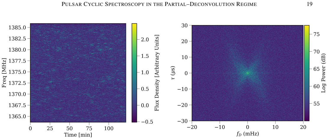
The paper's central claim is that complete phase retrieval is not the dividing line for the usefulness of cyclic spectroscopy. Using observations of three millisecond pulsars in both the full- and partial-deconvolution regimes, it shows that the squared modulus of a partially recovered dynamic wavefield, $|H(\nu,t)|^2$, reproduces the same scintillation pattern as the dynamic spectrum and yields nearly identical scintillation-bandwidth power-law fits, despite the wavefield phase being only partly recovered. Phase retrieval is found to be continuous: closer to the full-deconvolution boundary, more of the wavefield phase survives as signal structure rather than noise. The paper therefore concludes that partial-deconvolution data should be treated as incomplete rather than incorrect, and that cyclic processing is preferable to Fourier spectroscopy in all regimes when baseband data or a cyclic backend are available. It further claims that a modest cyclic merit can coexist with no observable deconvolution for low-flux, highly scattered pulsars, motivating a new predictor, cyclic merit 2.0, in which signal-to-noise is evaluated over a single scintillation bandwidth rather than the observing band; a power-law calibration maps the old threshold $m_{\rm cyc}\gg 1$ to $m_{\rm cyc,2.0}\gg 0.05$.
Load-bearing premise
The prediction of which pulsars will benefit rests on a power-law calibration between the old and new cyclic merits computed from one pulsar sample; if that mapping does not transfer to other telescopes, observing bands, or sources, the headline threshold of 0.05 and the source rankings would not hold.
Editorial extensions
If this is right
- Pulsar timing arrays can measure scattering delays for highly scattered pulsars even when full cyclic deconvolution fails, improving noise models and gravitational-wave sensitivity.
- Scintillation-bandwidth power-law studies of the interstellar medium can be done from dynamic wavefield power instead of dynamic spectra, with nearly identical measurements and extra harmonic information.
- Observing strategies should favor lower frequencies and highly scattered pulsars with narrow scintles, because phase recovery improves continuously toward the full-deconvolution boundary.
- Cyclic merit 2.0, once calibrated, lets observers rank pulsars by per-scintle signal-to-noise, exposing sources whose apparent merit is inflated by large scattering delay but whose faint flux per scintle makes deconvolution impractical.
- The upcoming availability of a cyclic spectroscopy backend would let observers obtain these benefits without retaining baseband data.
Reading between the lines
- The claim that dynamic wavefield power fully mirrors the dynamic spectrum in the partial regime could be quantified with a pixel-by-pixel residual statistic; testing this across many epochs would delimit exactly how complete the 'complete signal recovery' actually is.
- A natural prospective test is to pre-select pulsars predicted above the cyclic merit 2.0 threshold of 0.05, observe them, and compare deconvolution success rates against the old merit; this would validate or refute the transferability of the power-law calibration.
- The partial-recovery results suggest a hybrid pipeline the paper advocates but does not test: use cyclic spectroscopy to anchor the wavefield amplitude, and apply the $\theta-\theta$ transform only where its single-screen, anisotropic-scattering assumption holds, reserving cyclic partial phase for multi-screen lines of sight.
- Because the full-deconvolution boundary fluctuates with scintillation bandwidth from epoch to epoch, scheduling decisions could treat cyclic merit as a live observing metric rather than a static catalog value.
Signed reviews
Editorial analysis
A structured set of objections, weighed in public.
Referee Report
Summary. This paper investigates whether cyclic spectroscopy retains benefits for pulsar observations outside the full-deconvolution regime, where the scintillation bandwidth exceeds the inverse pulse width and complete recovery of the ISM transfer function is not possible. The authors analyze baseband observations of PSR B1937+21 (Arecibo ASP and PUPPI; GBT VEGAS), PSR J1643−1224, and PSR J1903+0327 (GBT), compute the cyclic figure of merit mcyc (Eq. 5) and full-deconvolution regime boundaries (Eq. 3), and extend these estimates to the NANOGrav 12.5-year pulsar sample under GBT and DSA-2000 sensitivities (Figs. 2–4). Comparing data products across regimes, they report that the partial-deconvolution dynamic wavefield contains coherent structure indicative of incomplete but genuine phase retrieval (Figs. 6–7); that dynamic wavefield power recovers the scintillation pattern and yields scintillation-bandwidth power-law fits nearly identical to those from the dynamic spectrum (Figs. 8–9); and that partial recovery of the secondary wavefield is possible, with the θ−θ transform discussed as a complementary approach (Figs. 10–11). Motivated by the null result for PSR J1903+0327—in the full-deconvolution regime yet with no discernible phase recovery—the paper introduces 'cyclic merit 2.0', based on scintillation rather than observing bandwidth, and uses a power-law fit (Fig. 18) to translate the original mcyc ≫ 1 threshold into mcyc,2.0 ≫ 0.05.
Significance. The central claim—that partial cyclic deconvolution still yields useful phase information and that dynamic wavefield power recovers the scintillation pattern in the partial-deconvolution regime—is practically important, since most NANOGrav pulsars are observed outside the full-deconvolution regime. If it holds, pulsar timing arrays could justify adopting cyclic processing for essentially all observations, with real gains in scattering-delay estimation and ISM studies. The survey-style merit and regime-boundary calculations for the full NANOGrav sample, with explicitly stated receiver and sky-temperature assumptions, are a genuinely useful planning resource for the GBT and DSA-2000. The paper's strengths include its detailed data products, its willingness to report the J1903+0327 null result, its explicit acknowledgment that part of the phase-imaginary resemblance is a small-angle effect, and its fair treatment of the θ−θ transform's limitations. The significance is currently capped by the absence of ground-truth or simulated validation of the partial-phase-retrieval claim, and by the under-specified, self-calibrated definition of cyclic merit 2.0.
major comments (4)
- [Section 5, definition of cyclic merit 2.0] Cyclic merit 2.0 is never defined by an equation. The text states that it 'behaves identical to the original cyclic merit' but 'relies on scintillation bandwidth rather than observing bandwidth' and that 'S/N now relies on flux density over a single scintle rather than the width of the observing band.' Since the original mcyc in Eq. (5) inherits its S/N from the bandwidth-dependent estimate of Eq. (8), the definition of mcyc,2.0 is ambiguous as written: exactly which bandwidth (full observing band, PFB channel, or scintillation bandwidth) enters the S/N term, and is the effective-pulse-width factor unchanged? Without an explicit formula, the values in Figs. 16–18 and the headline threshold are not reproducible. Please provide the full formula for mcyc,2.0 and state all assumptions used to compute it.
- [Section 5, Fig. 18] The decision threshold mcyc,2.0 ≫ 0.05 is obtained from a power-law fit between mcyc,2.0 and mcyc computed on the same NANOGrav sample with the same S/N model (Eq. 8) used to rank those same pulsars in Figs. 16 and 17. Because mcyc,2.0 is constructed from the same underlying quantities (scattering delay, S/N, pulse widths) as mcyc, the fit in Fig. 18 largely demonstrates self-correlation; it does not establish that mcyc,2.0 predicts deconvolution success on any independent outcome. No known-outcome test (e.g., the observations in Table 2 or a held-out set) is reported. The fit parameters, scatter, and residuals for Fig. 18 are not given, and the criterion as stated ('≫ 0.05') is non-operational: the paper does not state the mcyc,2.0 value corresponding to its own suggestion that mcyc ≳ 10 is sufficient. Given that the metric is motivated by the single J1903+0327 failure case, the 0.05 threshold should either be validated on independent outcomes or explicitly presented as a provisional calibration.
- [Section 4.2, Figs. 6–8] The central claim that genuine partial phase retrieval occurs rests on visual inspection of the recovered wavefields. In the partial-deconvolution regime the true H(ν,t) is unknown, so the coherent patches in Fig. 6 and the banded phase structure in Fig. 7 cannot be distinguished from regions of high S/N in which the iterative pycyc deconvolution converges to a stable but arbitrary phase. The paper itself notes in Section 4.2 that the phase and imaginary components resemble each other mainly because many recovered phases are near zero, which weakens the claim that non-trivial phase information is being recovered, and Section 4.3 reports non-physical power at negative delays in the partial-regime secondary wavefield. Moreover, the trend of more complete phase retrieval near the full-deconvolution regime (Fig. 7) is degenerate: observing frequency, S/N per scintle, and scattering delay vary together across the sub-bands, so the same trend would be expected even if the recovered phase were S/N-weighted noise. No simulation with an injected phase screen or quantitative phase-error measurement against the full-deconvolution control observation is provided. An end-to-end simulation with a known transfer function is needed to support the headline claim of partial phase retrieval, or the claim should be substantially softened.
- [Section 4.2, Fig. 9] The claim that the dynamic wavefield power shows 'complete signal recovery' in the partial-deconvolution regime is supported only by visual similarity to the dynamic spectrum (Fig. 8) and by the power-law fits of scintillation bandwidth versus frequency in Fig. 9. Such fits aggregate many scintles and are insensitive to pixel-level errors such as normalization offsets, smearing, or S/N-dependent bias, so they establish similar aggregate scintillation statistics but not faithful image recovery. Please either temper the 'complete signal recovery' wording or add a quantitative fidelity check, such as a cross-correlation or residual statistics between the dynamic spectrum and the wavefield power over the same time-frequency region.
minor comments (5)
- [Table 2] The 'a' note to the PSR J1903+0327 Δνd entry says the value was 'estimated from pulse broadening-inferred scattering delay'; please state explicitly how the conversion was made (presumably via Eq. 6 with C1 = 0.957) so the reader can propagate the uncertainty correctly.
- [Section 3.2] The pycyc iterative deconvolution is treated as a black box; a sentence on the update rule, initialization, number of iterations, and stopping criterion would materially aid reproducibility, particularly since the partial-regime results are interpreted as genuine phase recovery.
- [Section 3.4.1, Eq. (7)] The approximation Σk k² a_k ≈ (P/We)^{3/2} is stated without derivation; please cite the derivation in Turner et al. (2023) or give a brief justification of the step.
- [Fig. 8] The full- and partial-regime panels use different color scales (2–10 versus 1–6 in arbitrary units); a shared normalization or an explicit statement of the scales would make the claimed 'complete signal recovery' easier for the reader to judge.
- [Section 4.1.2, Figs. 2–4] The NANOGrav survey calculations depend on several assumed constants (C1 = 0.957, filling factor 0.2, and S/N bandwidths of 5/50/100 MHz); a brief sensitivity check of the merit rankings over the stated allowed ranges (e.g., C1 ∈ [0.6, 1.5]) would clarify how robust the conclusions in Figs. 2–4 are.
Circularity Check
Cyclic merit 2.0 threshold is fitted on the same NANOGrav sample it then labels, while the core partial-phase-retrieval analysis is independent.
-
fitted input called prediction
[Sec. 5 (Cyclic Merit 2.0) and Fig. 18; expectation labels in Figs. 16–17 captions.]
"To determine how cyclic merit 2.0 can be used to estimate the likelihood of successful cyclic deconvolution, we compared how a given pulsar’s calculated cyclic merit 1.0 differed from its corresponding cyclic merit 2.0 at a given observing frequency, with the results shown in Figure 18. By examining this behavior in log space, we can see that the resulting trend can be described quite well by a simple power law fit. When performing such an analysis in aggregate, our fit indicates that the original cyclic deconvolution threshold of mcyc≫ 1 translates to mcyc,2.0≫ 0.05."
Threshold 0.05 is obtained by a power-law fit to mcyc vs mcyc,2.0 computed for the same NANOGrav pulsars and same S/N model (Eq. 8) that are then ranked in Figs. 16–17, whose captions assert 'We would expect full cyclic deconvolution for sources with mcyc,2.0 ≫ 0.05.' The expectation is therefore a restatement of the fit, not an independent test against known deconvolution outcomes. The only external anchor, PSR J1903+0327's lack of results, is the same case that motivated the new metric, so its low 'assuringly' ranking is by construction. The metric is calibrated and then the calibrated values are used as evidence for the metric's usefulness. The independent partial-phase-retrieval demonstration is unaffected.
full rationale
The main load-bearing empirical claim—that partial-deconvolution cyclic spectroscopy recovers useful phase information and a useful dynamic wavefield power—is supported by direct comparisons of full- and partial-regime wavefields (Figs. 5–8) and by power-law fits of scintillation bandwidth from dynamic spectra versus dynamic wavefield power (Fig. 9). Those comparisons are not circular: the data products are constructed independently from the same baseband data, and no parameter is fitted from one product to force the other. The paper's reliance on prior work by the same authors (Dolch et al. 2021; Turner et al. 2023) is also not circular, because the cyclic merit formula and radical approximation are stated explicitly and applied rather than imported as an unexamined uniqueness theorem. The one genuine circularity is the calibration of the new cyclic merit 2.0 threshold: mcyc,2.0 ≫ 0.05 is obtained by a power-law fit between mcyc and mcyc,2.0 computed on the same NANOGrav pulsars and same S/N estimates that are then ranked and labeled 'expect full cyclic deconvolution' in Figs. 16–17. This is a self-calibration presented as a predictive threshold, and the only external failure case (PSR J1903+0327) is the same case used to motivate the metric. That makes the source-ranking and threshold component partially circular, even though the partial-phase-retrieval result stands independently. Score 6 reflects that the central demonstration is independent but one 'prediction' (the mcyc,2.0 expectation threshold) reduces to its own fit.
Assumptions & free parameters
free parameters (5)
- C1 conversion constant =
0.957
- Assumed S/N bandwidths for NANOGrav survey =
5 MHz at 350 MHz, 50 MHz at 820 MHz, 100 MHz at 1500 MHz
- Filling factors for scintle count =
eta_nu = eta_t = 0.2
- Scintillation scaling indices =
nu^4.4 for bandwidth, nu^1.2 for timescale
- Cyclic merit 2.0 decision threshold =
0.05 (mcyc,2.0 much greater than 0.05)
assumptions (6)
- domain assumption The observed cyclic spectrum factorizes as SE(nu, alpha_k) = <H(nu+alpha_k/2)H*(nu-alpha_k/2)> Sx(nu, alpha_k) (Eq. 2), separating the ISM transfer function from the intrinsic pulse.
- domain assumption Full cyclic deconvolution is possible when Delta_nu_d is less than or about 1/W10 (Eq. 3).
- domain assumption Scattering delay can be estimated from scintillation bandwidth by Delta_nu_d = C1/(2 pi tau_d) with C1 = 0.957 (Eq. 6).
- domain assumption The radiometer equation (Eq. 8) with assumed telescope gain, system temperature, and bandwidth gives a valid S/N estimate for each NANOGrav pulsar.
- domain assumption Scintillation bandwidth and timescale scale as nu^4.4 and nu^1.2 across observing frequencies.
- domain assumption The theta-theta transform requires a single anisotropic phase screen to recover the secondary wavefield.
Cite this review
Pith. "Pith review of Pulsar Cyclic Spectroscopy in the Partial-Deconvolution Regime: Benefits & Limitations." pith.science (2026). https://pith.science/paper/TPWEEOLN
@misc{pith2026250513832,
  author       = {Pith},
  title        = {Pith review of: Pulsar Cyclic Spectroscopy in the Partial-Deconvolution Regime: Benefits & Limitations},
  year         = {2026},
  howpublished = {\url{https://pith.science/paper/TPWEEOLN}},
  note         = {Machine review of arXiv:2505.13832}
}
abstract
We explore possible advantages of cyclic spectroscopy for observations of pulsars in instances where full cyclic deconvolution is not feasible. We compute cyclic merits and full-deconvolution regime boundaries for pulsars observed by NANOGrav and discuss which sources stand to benefit the most from using cyclic spectroscopy when observed with the Green Bank Telescope and DSA-2000 in a given frequency range. We compare data products, namely the wavefield, in both full-deconvolution and partial-deconvolution regimes to demonstrate what can be accomplished with incomplete phase retrieval. Additionally, we show how some phase retrieval can still be achieved in the partial-deconvolution regime and how this allows for additional information in scintillation-based data products, like the dynamic wavefield power, compared to what can be found in traditional dynamic spectra. An examination of dynamic wavefield phase as a function of observing frequency reveals more complete phase retrieval is achieved the closer one gets to the full deconvolution regime, agreeing with the expectations of cyclic merit. While we demonstrate that fragmentary recovery of the secondary wavefield can be accomplished in the partial-deconvolution regime, we advocate for a synergistic approach with phase retrieval methods like the $\theta-\theta$ transform, although we also provide discussion about shortcomings of this strategy. Finally, we use the combination of modest cyclic merit and lack of discernible results for PSR J1903$+$0327 to motivate the creation of an updated "cyclic merit 2.0", which relies on scintillation bandwidth instead of observing bandwidth.
Figures


Figures from the paper (15 more)




Reference graph
Works this paper leans on
-
[1]
, " * write output.state after.block = add.period write newline
ENTRY address archivePrefix author booktitle chapter doi edition editor eprint howpublished institution journal key month number organization pages publisher school series title misctitle type volume year version url label extra.label sort.label short.list INTEGERS output.state before.all mid.sentence after.sentence after.block FUNCTION init.state.consts ...
-
[2]
write newline
" write newline "" before.all 'output.state := FUNCTION format.url url empty "" new.block "" url * "" * if FUNCTION format.eprint eprint empty "" archivePrefix empty "" archivePrefix "arXiv" = new.block " " eprint * " " * new.block " " eprint * " " * if if if FUNCTION format.doi doi empty "" " " doi * " " * if FUNCTION format.pid doi empty eprint empty ur...
-
[3]
," = swap duplicate
thebibliography [1] 20pt to REFERENCES 6pt =0pt 10pt plus 3pt =0pt =0pt =1pt plus 1pt =0pt =0pt -12pt =13pt plus 1pt =20pt =13pt plus 1pt \@M =10000 =-1.0em =0pt =0pt 0pt =0pt =1.0em @enumiv\@empty 10000 10000 `\.\@m \@noitemerr \@latex@warning Empty `thebibliography' environment \@ifnextchar \@reference \@latexerr Missing key on reference command Each re...
2019
-
[4]
write newline
" write newline "" before.all 'output.state := FUNCTION new.block output.state before.all = 'skip after.block 'output.state := if FUNCTION field.or.null duplicate empty pop "" 'skip if FUNCTION format.annotation annotation empty "" " quotation " annotation * " quotation " * if FUNCTION fin.entry note output write newline format.annotation write INTEGERS n...
-
[5]
, " * write output.state after.block = add.period write newline
ENTRY address archivePrefix author booktitle chapter doi edition editor eprint howpublished institution journal key month note number organization pages publisher school series title type volume year label extra.label sort.label short.list INTEGERS output.state before.all mid.sentence after.sentence after.block FUNCTION init.state.consts #0 'before.all :=...
-
[6]
write newline
" write newline "" before.all 'output.state := FUNCTION format.doi doi empty "" "doi:" doi * if FUNCTION format.eprint eprint empty "" archivePrefix empty "" archivePrefix ":" * if eprint field.or.null * if FUNCTION format.pid eprint empty format.doi format.eprint if FUNCTION n.dashify 't := "" t empty not t #1 #1 substring "-" = t #1 #2 substring "--" = ...
-
[7]
write newline
" write newline "" before.all 'output.state := FUNCTION format.archive archivePrefix empty "" archivePrefix ":" * if FUNCTION format.primaryClass primaryClass empty "" " [" primaryClass * "]" * if FUNCTION format.eprint eprint empty pages empty not booktitle empty not or or "" archive empty " http://arxiv.org/abs/" eprint * " " * " " * format.archive * ep...
-
[8]
Agazie, G., Alam, M. F., Anumarlapudi, A., et al. 2023 a , The Astrophysical Journal Letters, 951, L9, 10.3847/2041-8213/acda9a
Show all 54 references
-
[9]
M., et al
Agazie, G., Anumarlapudi, A., Archibald, A. M., et al. 2023 b , ApJL, 951, L10, 10.3847/2041-8213/acda88
2023 doi
-
[10]
F., Arzoumanian, Z., Baker, P
Alam, M. F., Arzoumanian, Z., Baker, P. T., et al. 2020, The Astrophysical Journal Supplement Series, 252, 4, 10.3847/1538-4365/abc6a0
2020 doi
-
[11]
P., Tollerud , E
Astropy Collaboration , Robitaille , T. P., Tollerud , E. J., et al. 2013, , 558, A33, 10.1051/0004-6361/201322068
2013 doi
-
[12]
H., et al
Baker , D., Brisken , W., van Kerkwijk , M. H., et al. 2022, , 510, 4573, 10.1093/mnras/stab3599
2022 doi
-
[13]
H., van Lieshout, R., & Pen, U.-L
Baker, D., Brisken, W., van Kerkwijk, M. H., van Lieshout, R., & Pen, U.-L. 2023, Monthly Notices of the Royal Astronomical Society, 525, 211, 10.1093/mnras/stad2318
2023 doi
-
[14]
D., et al
Burgay , M., Bailes , M., Bates , S. D., et al. 2013, , 433, 259, 10.1093/mnras/stt721
2013 doi
-
[15]
Cordes, J. M. 1986, ApJ, 311, 183, 10.1086/164764
1986 doi
-
[16]
M., & Lazio, T
Cordes, J. M., & Lazio, T. J. W. 2002, NE2001.I. A New Model for the Galactic Distribution of Free Electrons and its Fluctuations
2002
- [17]
-
[18]
M., Weisberg , J
Cordes , J. M., Weisberg , J. M., & Boriakoff , V. 1985, , 288, 221, 10.1086/162784
1985 doi
-
[21]
S., McLaughlin , M., Olszanski , T
Deneva , J. S., McLaughlin , M., Olszanski , T. E. E., et al. 2024, , 271, 23, 10.3847/1538-4365/ad19da
2024 doi
-
[22]
R., Jones, G., et al
Dolch, T., Stinebring, D. R., Jones, G., et al. 2021, ApJ, 913, 98, 10.3847/1538-4357/abf48b
2021 doi
-
[23]
B., Schinzel , F
Dowell , J., Taylor , G. B., Schinzel , F. K., Kassim , N. E., & Stovall , K. 2017, , 469, 4537, 10.1093/mnras/stx1136
2017 doi
-
[24]
M., Lam, M
Geiger, A., Cordes, J. M., Lam, M. T., et al. 2025, The Astrophysical Journal, 986, 191, 10.3847/1538-4357/add0b6
2025 doi
-
[25]
J., & Gaensler, B
Harvey-Smith, L., Madsen, G. J., & Gaensler, B. M. 2011, The Astrophysical Journal, 736, 83, 10.1088/0004-637X/736/2/83
2011 doi
-
[26]
Hunter, J. D. 2007, CSE, 9, 90, 10.1109/MCSE.2007.55
2007 doi
-
[27]
A., Bailes, M., Ord, S
Jacoby, B. A., Bailes, M., Ord, S. M., Knight, H. S., & Hotan, A. W. 2007, The Astrophysical Journal, 656, 408, 10.1086/509312
2007 doi
-
[28]
Lam , M. T. 2017, PyPulse: PSRFITS handler . 1706.011
2017
-
[29]
T., McLaughlin, M
Lam, M. T., McLaughlin, M. A., Arzoumanian, Z., et al. 2019, ApJ, 872, 193, 10.3847/1538-4357/ab01cd
2019 doi
-
[30]
A., Jones, G., et al
Levin, L., McLaughlin, M. A., Jones, G., et al. 2016, ApJ, 818, 166. http://stacks.iop.org/0004-637X/818/i=2/a=166
2016
-
[31]
Liu , Y., Verbiest , J. P. W., Main , R. A., et al. 2022, , 664, A116, 10.1051/0004-6361/202142552
2022 doi
-
[32]
Mahajan, N., & van Kerkwijk, M. H. 2023, The Astrophysical Journal, 955, 33, 10.3847/1538-4357/acec3a
2023 doi
-
[33]
A., Antoniadis, J., Chen, S., et al
Main, R. A., Antoniadis, J., Chen, S., et al. 2023, Monthly Notices of the Royal Astronomical Society, 525, 1079, 10.1093/mnras/stad1980
2023 doi
-
[34]
A., Antoniadis, J., et al
Mall, G., Main, R. A., Antoniadis, J., et al. 2022, Monthly Notices of the Royal Astronomical Society, 511, 1104, 10.1093/mnras/stac096
2022 doi
-
[35]
E., Spiewak , R., Swiggum , J
McEwen , A. E., Spiewak , R., Swiggum , J. K., et al. 2020, , 892, 76, 10.3847/1538-4357/ab75e2
2020 doi
-
[36]
K., Cordes, J
Ocker, S. K., Cordes, J. M., & Chatterjee, S. 2020, The Astrophysical Journal, 897, 124, 10.3847/1538-4357/ab98f9
2020 doi
-
[37]
K., Cordes, J
Ocker, S. K., Cordes, J. M., Chatterjee, S., et al. 2023, Monthly Notices of the Royal Astronomical Society, 527, 7568, 10.1093/mnras/stad3683
2023 doi
-
[38]
Price , D. C. 2016, PyGDSM: Python interface to Global Diffuse Sky Models , Astrophysics Source Code Library, record ascl:1603.013
2016
-
[39]
J., Coles , W
Reardon , D. J., Coles , W. A., Bailes , M., et al. 2020, , 904, 104, 10.3847/1538-4357/abbd40
2020 doi
-
[40]
J., Bigot-Sazy , M
Remazeilles , M., Dickinson , C., Banday , A. J., Bigot-Sazy , M. A., & Ghosh , T. 2015, , 451, 4311, 10.1093/mnras/stv1274
2015 doi
-
[41]
2021, , 500, 1114, 10.1093/mnras/staa3353
Sprenger , T., Wucknitz , O., Main , R., Baker , D., & Brisken , W. 2021, , 500, 1114, 10.1093/mnras/staa3353
2021 doi
-
[42]
H., Thorsett , S
Stairs , I. H., Thorsett , S. E., & Camilo , F. 1999, , 123, 627, 10.1086/313245
1999 doi
-
[43]
R., McLaughlin , M
Stinebring , D. R., McLaughlin , M. A., Cordes , J. M., et al. 2001, , 549, L97, 10.1086/319133
2001 doi
-
[44]
E., Stinebring , D
Turner , J. E., Stinebring , D. R., McLaughlin , M. A., et al. 2023, , 944, 191, 10.3847/1538-4357/acb6fd
2023 doi
-
[45]
E., McLaughlin , M
Turner , J. E., McLaughlin , M. A., Cordes , J. M., et al. 2021, , 917, 10, 10.3847/1538-4357/abfafe
2021 doi
-
[46]
E., Dolch, T., Cordes, J
Turner, J. E., Dolch, T., Cordes, J. M., et al. 2024, The Astrophysical Journal, 972, 16, 10.3847/1538-4357/ad5af9
2024 doi
-
[47]
C., & Varoquaux , G
van der Walt , S., Colbert , S. C., & Varoquaux , G. 2011, CSE, 13, 22
2011
-
[48]
2011, , 28, 1, 10.1071/AS10021
van Straten , W., & Bailes , M. 2011, , 28, 1, 10.1071/AS10021
2011 doi
-
[49]
A., Demorest, P
Walker, M. A., Demorest, P. B., & van Straten, W. 2013, The Astrophysical Journal, 779, 99, 10.1088/0004-637X/779/2/99
2013 doi
-
[50]
A., Koopmans, L
Walker, M. A., Koopmans, L. V. E., Stinebring, D. R., & Van Straten, W. 2008, Monthly Notices of the Royal Astronomical Society, 388, 1214, 10.1111/j.1365-2966.2008.13452.x
2008
-
[51]
A., & Stinebring , D
Walker , M. A., & Stinebring , D. R. 2005, , 362, 1279, 10.1111/j.1365-2966.2005.09396.x
2005
-
[52]
F., Han , J
Wang , P. F., Han , J. L., Xu , J., et al. 2023, Research in Astronomy and Astrophysics, 23, 104002, 10.1088/1674-4527/acea1f
2023 doi
-
[53]
2024, , 961, 48, 10.3847/1538-4357/ad0724
Wang , X.-W., Yan , Z., Shen , Z.-Q., et al. 2024, , 961, 48, 10.3847/1538-4357/ad0724
2024 doi
-
[54]
M., Manchester , R
Yan , W. M., Manchester , R. N., van Straten , W., et al. 2011, , 414, 2087, 10.1111/j.1365-2966.2011.18522.x
2011
-
[55]
Young, O., & Lam, M. T. 2024, The Astrophysical Journal, 962, 131, 10.3847/1538-4357/ad1ce7
2024 doi
-
[56]
S., et al
Zheng , H., Tegmark , M., Dillon , J. S., et al. 2017, , 464, 3486, 10.1093/mnras/stw2525
2017 doi
Reviewed August 15, 2026 · model on record in the stance chip above.
Discussion (0). Continue with ORCID to comment.