REVIEW 3 major objections 4 minor 1 cited by
An Adaptive-rank Approach with Greedy Sampling for Multi-scale BGK Equations
T0 review · 3 major / 4 minor · reviewed 2026-08-07 · deepseek-v4-flash
Pith's one-line read An adaptive-rank BGK scheme conserves mass, momentum, and energy to machine precision while capturing fluid-kinetic regimes.
desk verdict Promising low-rank BGK solver with strong numerics; the conditional AP theorem's proof is circular and needs rework before the theoretical claims are cited. read the letter →
The pith
A machine-rendered reading of the paper's core claim, the machinery that carries it, and where it could break.
The reading
What carries the argument
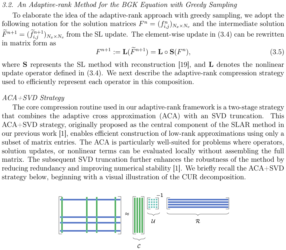
The load-bearing object is the ACA+SVD compression routine, in which adaptive cross approximation builds a CUR decomposition $A\approx A(:,J)A(I,J)^{-1}A(I,:)$ by greedily choosing pivots from the residual, followed by an SVD truncation that removes redundant modes. Applied once to the semi-Lagrangian characteristic update and once to the BGK relaxation update, the routine updates only the selected rows and columns, so the local Maxwellian is evaluated pointwise at sample locations rather than decomposed. The second carrying mechanism is the locally macroscopic conservative (LoMaC) correction, an implicit coupling of the low-rank kinetic solution to a macroscopic moment system whose flux is closed dynamically by the kinetic solution; the resulting nonlinear system is solved by a Jacobian-free Newton-Krylov method with the provisional solution as initial guess.
What would settle it
On a benchmark whose fluid limit has small numerical rank (so Corollary 3.7's condition is met), set the truncation tolerances to $\epsilon_c=\epsilon_s=\epsilon$, take one time step at CFL 4, and measure $\lVert F^{n+1}-M_U(F^{n+1})\rVert_\infty$ as $\epsilon\to 0$. If the deviation does not decay like $O(\epsilon)$, the conditional asymptotic-preserving claim fails even where its assumptions hold.
Extended reading notes
Core claim
The central claim is that greedy sampling plus SVD truncation can carry the full multi-scale behavior of the BGK equation without explicit low-rank decompositions of its nonlinear collision term. After a provisional nonconservative low-rank update $F^{n+1,\star}$, the LoMaC correction imposes conservation through $F^{n+1}=F^{n+1,\star}-M_{U(F^{n+1,\star})}+M_{U^{n+1}}$, where $U^{n+1}$ solves an implicit, stiffly accurate DIRK discretization of the macroscopic flux system with a kinetic-flux-splitting space discretization. The asymptotic analysis proves that the full-grid scheme's asymptotic-preserving and asymptotically accurate behavior survives the correction (Theorem 3.5), and that the low-rank scheme is conditionally asymptotically accurate when the combined CUR and SVD truncation errors are $O(\epsilon)$ (Corollary 3.7). Numerical studies show third-order temporal and spatial convergence for Knudsen numbers from $10^{-6}$ to $10^{-2}$, correct shock and rarefaction structures, and stable behavior on a mixed-regime problem with space-varying Knudsen number.
Load-bearing premise
The load-bearing premise is that the combined CUR and SVD truncation error is $O(\epsilon)$ as the Knudsen number goes to zero, which is not automatic because a generic local Maxwellian does not have low rank.
Editorial extensions
If this is right
- Mass, momentum, and energy are conserved to machine precision despite low-rank compression.
- Large CFL numbers are feasible: CFL 4 is used throughout the numerical tests, with small Newton and Krylov iteration counts and no preconditioning at moderate CFL.
- The scheme captures shocks, contact discontinuities, and rarefactions across Knudsen numbers from $10^{-6}$ to $10^{-2}$.
- For mixed regimes in which the Knudsen number varies over six orders of magnitude, the solution rank stays modest, using roughly 15–23% of full-grid storage.
- With truncation tolerances chosen $O(\epsilon)$, the low-rank scheme inherits the asymptotic-preserving property of the underlying full-grid semi-Lagrangian method.
Reading between the lines
- If the distribution is written multiplicatively as $f=M_{U(f)}g$, the limiting fluid solution has rank one, which would likely turn the conditional asymptotic-preserving guarantee into an unconditional one; the authors explicitly leave this variant for future work.
- The pointwise-evaluation trick for the local Maxwellian may transfer to other stiff kinetic operators, such as Fokker-Planck or full Boltzmann collisions, wherever the nonlinear term can be evaluated locally without low-rank assembly.
- A scaling study of the observed rank versus $\epsilon$ at fixed error tolerance would show where the method's efficiency advantage starts to degrade, since a generic local Maxwellian is not low rank.
- The moment correction behaves like a dynamic closure; it would be worth testing whether it also damps spurious oscillations of the low-rank solution in strongly non-equilibrium regions.
Editorial analysis
A structured set of objections, weighed in public.
Referee Report
Summary. The paper proposes an adaptive-rank numerical method for the multi-scale BGK equation. The method combines a greedy adaptive cross approximation (ACA) with SVD truncation, a local semi-Lagrangian finite-difference solver, and a locally macroscopic conservative (LoMaC) correction that enforces mass, momentum, and energy conservation by implicitly coupling the kinetic solution to a macroscopic moment system. High-order temporal accuracy is obtained with stiffly accurate DIRK methods, and the resulting nonlinear systems are solved with a Jacobian-free Newton-Krylov method. The main theoretical claims are that the LoMaC correction preserves the asymptotic-preserving (AP) and asymptotically accurate (AA) properties of the full-grid scheme, and that the low-rank scheme is conditionally AP provided certain truncation errors are O(epsilon) (Theorem 3.6 and Corollary 3.7). Numerical experiments report third-order temporal and spatial convergence for a range of Knudsen numbers, machine-precision conservation, and robust behavior on a Riemann problem and a mixed-regime problem with spatially varying Knudsen number.
Significance. If the theoretical claims are sound, the paper makes a useful contribution: it extends the semi-Lagrangian adaptive-rank framework to collisional kinetic equations without forming explicit low-rank decompositions of the local Maxwellian, and it demonstrates strict conservation of all three collision invariants. The numerical evidence is strong: the convergence tables are clean, conservation is attained to machine precision across all tested regimes, and the mixed-regime experiments show stable behavior over several orders of magnitude of the Knudsen number. The authors are also transparent about limitations, including the conditional nature of the AP result and the difficulty of controlling accumulated truncation error. However, the central asymptotic analysis, specifically the proof of Theorem 3.6, contains a load-bearing gap that affects Corollary 3.7 and therefore the paper's main theoretical claim. The numerical experiments are convincing as algorithmic demonstrations, but they do not currently close that gap.
major comments (3)
- [§3.5, Theorem 3.6] The proof of Theorem 3.6 is circular and does not establish the stated bound. After the LoMaC correction (3.23), the moments of F^(k) are enforced to equal U^(k), so M_U(F^(k)) = M_{U^(k)} and (3.23) gives F^(k) - M_U(F^(k)) = F^(k),*_{#,k2->r2} - M_U(F^(k),*_{#,k2->r2}). The first term in the decomposition (3.27) is therefore exactly the quantity the theorem is supposed to bound. The sentence preceding (3.28), which asserts that 'the initial data is well-prepared and the local solver is AA' implies the bound, applies the full-grid AA result of [20] to the truncated provisional solution, for which that result is not proven. In addition, the two E-terms in (3.29) sum to F^(k),*_{#,k2->r2} - F^(k), which by (3.23) equals the LoMaC adjustment M_U(F^(k),*_{#,k2->r2}) - M_{U^(k)}; they do not include the S-stage truncation error, and the discussion after (3.31) concedes that this accumulation is difficult to control. Consequently, Corollary 3.7 imposes its O(epsilon) condition on quantities that can be small while F^(k) - M_U(F^(k)) is large, so the conditional AP/AA property is not established by the present argument.
- [Corollary 3.7 and Remark 3.8] Even if Theorem 3.6 were repaired, the conditional AP property as stated is substantially weaker than the abstract suggests. The condition ||E_eps_s(F^(k)_{#,k2})|| + ||E_eps_c(F^(k))|| lesssim epsilon forces the truncation tolerances to scale with the Knudsen number, and Remark 3.8 admits that this may require large ranks and undermine efficiency. The generic fluid limit has a local Maxwellian that is not low-rank in the x-v tensor format except under rank-degeneracy or special assumptions. The numerical tests in Section 4 use fixed tolerances (for example, epsilon_C = 1e-9 and epsilon_S = 1e-8 in Example 4.1, and much looser tolerances in Example 4.2) and do not demonstrate that the Corollary's condition is satisfied. The manuscript should clarify whether Corollary 3.7 is intended as a proof of a practical AP property or as a consistency condition that practical tolerance choices must satisfy.
- [Theorem 3.4 and numerical tests] The AP/AA analysis assumes well-prepared initial data (Definition 3.3) and exact spatial interpolation at the characteristic feet, as stated in Theorem 3.4. The numerical experiments use WENO spatial reconstruction and, in Example 4.2, discontinuous Riemann initial data, so the theory does not cover the regimes in which the method is actually tested. The authors are transparent about these restrictions, but the manuscript should state explicitly that the numerical evidence is heuristic support for the method rather than verification of the conditional AP theorem in the tested configurations.
minor comments (4)
- [§3.3.1] The expression 'eR R± ·dv' in the text after equation (3.14) appears to be a rendering artifact; it should read as an integral over the half-velocity domains, e.g., ∫_{R±} · dv.
- [Example 4.2] In the sentence 'Our results indicate that smaller values of epsilon generally lead to an SLightly higher number of iterations', 'SLightly' should be 'slightly'.
- [Remark 3.9] Remark 3.9 refers to 'Theorem 3.7', but the conditional AA property is stated in Corollary 3.7; the cross-reference should be corrected.
- [Notation in Section 3.3 and 3.5] The notation M_U(F^(k)) versus M_{U^(k)} is used without explicit definition of the latter; since the distinction between 'Maxwellian with moments of the provisional solution' and 'Maxwellian with the enforced macroscopic moments' is central to the LoMaC correction, a short notational clarification would improve readability.
Circularity Check
Theorem 3.6's asymptotic bound is asserted rather than proved: the LoMaC identity forces the target deviation to equal the provisional low-rank deviation, and the proof then assumes that deviation is O(ε).
-
self definitional
[Section 3.5, Theorem 3.6 proof, Eqs. (3.27)–(3.28)]
"F^(k) − M_U(F^(k)) = F^(k),⋆_{#,k2→r2} − M_U(F^(k),⋆_{#,k2→r2}) = F^(k) − M_U(F^(k)) + F^(k),⋆_{#,k2→r2} − F^(k) + M_U(F^(k)) − M_U(F^(k),⋆_{#,k2→r2}). ... Since the initial data is well-prepared and the local solver is AA, then we immediately have that ‖F^(k) − M_U(F^(k))‖ ≲ ε."
By the LoMaC definition (3.23), F^(k) = F^(k),⋆ − M_U(F^(k),⋆) + M_{U^(k)}; taking moments shows M_U(F^(k)) = M_{U^(k)}, hence F^(k) − M_U(F^(k)) = F^(k),⋆ − M_U(F^(k),⋆) exactly. Thus the first line of (3.27) reduces the theorem's target quantity to the deviation of the truncated provisional solution from its own Maxwellian. The sentence preceding (3.28) then asserts that this very deviation is O(ε) by citing the full-grid AA property of [20]; but [20] applies to the untruncated scheme, not to the ACA/SVD-truncated F^(k),⋆, and no bound on the S-stage truncation error is supplied.
full rationale
The numerical conservation results are genuine and not circular: conservation is enforced by construction through the LoMaC macroscopic correction and the conservative finite-volume discretization, so reporting machine-precision conservation is self-consistent. The dependence on [20] for the full-grid AP/AA property and on [1] for ACA+SVD compression is standard prior work and is not by itself circular. The significant issue is Theorem 3.6: the proof's decomposition (3.27) is an identity that rewrites the target deviation as the provisional low-rank deviation, and the bound (3.28) is then asserted from the full-grid AA property, which does not apply to the truncated solution. Because the S-stage truncation error is omitted from the stated bound (as conceded after (3.31)), Corollary 3.7's O(ε) condition controls the wrong terms and does not establish the claimed conditional AP property. This is a partial circularity/gap in the central analytic claim, not in the numerical scheme itself; hence score 6.
Assumptions & free parameters
free parameters (5)
- CUR truncation tolerance epsilon_C =
1e-9, 1e-4, 1e-8 in different tests
- SVD truncation tolerance epsilon_S =
1e-8, 1e-3, 1e-7 in different tests
- Newton tolerance =
1e-14
- Krylov tolerance =
1e-6
- CFL number =
1 to 4 depending on the test
assumptions (4)
- domain assumption The full-grid SL-FD scheme from [19,20] is asymptotic-preserving and asymptotically accurate for the BGK equation.
- domain assumption Initial data are well-prepared in the sense of Definition 3.3.
- domain assumption Exact spatial interpolation is used at the feet of the characteristics.
- domain assumption The density and temperature are bounded away from zero so that the Maxwellian Jacobian is bounded.
Cite this review
Pith. "Pith review of An Adaptive-rank Approach with Greedy Sampling for Multi-scale BGK Equations." pith.science (2026). https://pith.science/paper/IXPT7DAX
@misc{pith2026250517191,
  author       = {Pith},
  title        = {Pith review of: An Adaptive-rank Approach with Greedy Sampling for Multi-scale BGK Equations},
  year         = {2026},
  howpublished = {\url{https://pith.science/paper/IXPT7DAX}},
  note         = {Machine review of arXiv:2505.17191}
}
read the original abstract
In this paper, we propose a novel adaptive-rank method for simulating multi-scale BGK equations, based on a greedy sampling strategy. The method adaptively selects important rows and columns of the solution matrix and updates them using a local semi-Lagrangian solver. An adaptive cross approximation then reconstructs the full solution matrix. This extends our prior semi-Lagrangian adaptive-rank framework, developed for the Vlasov-Poisson system, to nonlinear collisional kinetic equations. Unlike step-and-truncate low-rank integrators, our greedy sampling approach avoids explicit low-rank decompositions of nonlinear terms, such as the local Maxwellian in the BGK operator. To ensure conservation, we introduce a locally macroscopic conservative correction that implicitly couples the kinetic and macroscopic systems, enforcing mass, momentum, and energy conservation. Through asymptotic analysis, we show that this correction preserves the full-grid scheme's asymptotic behavior, and that the proposed method is conditionally asymptotic-preserving in the low-rank setting. A key advantage of our approach is its use of a local semi-Lagrangian solver, which allows large time steps. This flexibility is retained in the macroscopic solver using high-order stiffly accurate diagonally implicit Runge-Kutta methods. The resulting nonlinear systems are solved efficiently using a Jacobian-free Newton-Krylov method, avoiding the need for preconditioning at modest CFL numbers. Each nonlinear iteration provides a self-consistent correction to a provisional kinetic solution, which serves as a dynamic closure for the macroscopic model. Numerical results demonstrate the method's accuracy in capturing shocks and its robustness across mixed-regime problems with wide-ranging Knudsen numbers.
Figures


Figures from the paper (15 more)


Forward citations
Cited by 1 Pith paper
-
A Nodal Discontinuous Galerkin Method with Rank-Adaptive Velocity Space Representation for the Multiscale BGK Model
A full-rank-in-space, low-rank-in-velocity nodal DG solver for 1d2v BGK is shown to be high-order, conservative, and asymptotic-preserving, with complexity linear in the velocity grid size.
Reference graph
Works this paper leans on
-
[20]
M. Ding, J.-M. Qiu, R. Shu, Accuracy and stability analysis of the semi-lagrangian method for stiff hyperbolic relaxation systems and kinetic BGK model, SIAM Multiscale Modeling & Simulation 21 (1) (2023) 143–167
work page 2023
- [1]
-
[2]
L. Einkemmer, K. Kormann, J. Kusch, R. G. McClarren, J.-M. Qiu, A review of low- rank methods for time-dependent kinetic simulations, Journal of Computational Physics (2025) 114191
work page 2025
-
[3]
P. Bhatnagar, E. Gross, M. Krook, A model for collision processes in gases. I. small amplitude processes in charged and neutral one-component systems, Physical review 94 (3) (1954) 511
work page 1954
-
[4]
O. Koch, C. Lubich, Dynamical low-rank approximation, SIAM Journal on Matrix Analysis and Applications 29 (2) (2007) 434–454
2007
-
[5]
L. Einkemmer, C. Lubich, A low-rank projector-splitting integrator for the Vlasov– Poisson equation, SIAM Journal on Scientific Computing 40 (5) (2018) B1330–B1360
work page 2018
-
[6]
L. Einkemmer, A low-rank algorithm for weakly compressible flow, SIAM Journal on Scientific Computing 41 (5) (2019) A2795–A2814
work page 2019
-
[7]
L. Einkemmer, J. Hu, L. Ying, An efficient dynamical low-rank algorithm for the Boltzmann-BGK equation close to the compressible viscous flow regime, SIAM Journal on Scientific Computing 43 (5) (2021) B1057–B1080
work page 2021
Show all 39 references
-
[8]
Ceruti, C
G. Ceruti, C. Lubich, An unconventional robust integrator for dynamical low-rank ap- proximation, BIT Numerical Mathematics 62 (1) (2022) 23–44
2022
-
[9]
Baumann, L
L. Baumann, L. Einkemmer, C. Klingenberg, J. Kusch, A stable multiplicative dy- namical low-rank discretization for the linear Boltzmann-BGK equation, arXiv preprint arXiv:2411.06844 (2024)
2024 arXiv
-
[10]
Kormann, A semi-Lagrangian Vlasov solver in tensor train format, SIAM Journal on Scientific Computing 37 (4) (2015) B613–B632
K. Kormann, A semi-Lagrangian Vlasov solver in tensor train format, SIAM Journal on Scientific Computing 37 (4) (2015) B613–B632
2015
-
[11]
Dektor, A
A. Dektor, A. Rodgers, D. Venturi, Rank-adaptive tensor methods for high-dimensional nonlinear PDEs, Journal of Scientific Computing 88 (2) (2021) 36
2021
-
[12]
Guo, J.-M
W. Guo, J.-M. Qiu, A low rank tensor representation of linear transport and nonlinear Vlasov solutions and their associated flow maps, Journal of Computational Physics 458 (2022) 111089. doi:111089
2022
-
[13]
W. Guo, J. F. Ema, J.-M. Qiu, A Local Macroscopic Conservative (LoMaC) low rank tensor method with the discontinuous Galerkin method for the Vlasov dynamics, Com- munications on Applied Mathematics and Computation 6 (1) (2024) 550–575. 31
2024
-
[14]
W. A. Sands, W. Guo, J.-M. Qiu, T. Xiong, High-order adaptive rank integrators for multi-scale linear kinetic transport equations in the hierarchical Tucker format, SIAM Journal on Scientific Computing (to appear) (2025)
2025
-
[15]
T. Shi, D. Hayes, J.-M. Qiu, Distributed memory parallel adaptive tensor-train cross approximation, arXiv preprint arXiv:2407.11290 (2024)
2024 arXiv
-
[16]
Dektor, Collocation methods for nonlinear differential equations on low-rank mani- folds, Linear Algebra and its Applications 705 (2025) 143–184
A. Dektor, Collocation methods for nonlinear differential equations on low-rank mani- folds, Linear Algebra and its Applications 705 (2025) 143–184
2025
-
[17]
Dektor, L
A. Dektor, L. Einkemmer, Interpolatory dynamical low-rank approximation for the 3+ 3d Boltzmann-BGK equation, arXiv preprint arXiv:2411.15990 (2024)
2024 arXiv
-
[18]
Guo, J.-M
W. Guo, J.-M. Qiu, A conservative low rank tensor method for the Vlasov dynamics, SIAM Journal on Scientific Computing 46 (1) (2024) A232–A263
2024
-
[19]
L. Li, J. Qiu, G. Russo, A high-order semi-Lagrangian finite difference method for non- linear Vlasov and BGK models, Communications on Applied Mathematics and Com- putation 5 (1) (2023) 170–198
2023
-
[21]
W. T. Taitano, D. A. Knoll, L. Chacón, J. M. Reisner, A. K. Prinja, Moment-based acceleration for neutral gas kinetics with BGK collision operator, Journal of Computa- tional and Theoretical Transport 43 (1-7) (2014) 83–108
2014
-
[22]
W. T. Taitano, D. A. Knoll, L. Chacón, Charge-and-energy conserving moment-based accelerator for a multi-species Vlasov–Fokker–Planck–Ampère system, part II: Colli- sional aspects, Journal of Computational Physics 284 (2015) 737–757
2015
-
[23]
H. Park, L. Chacón, A. Matsekh, G. Chen, A multigroup moment-accelerated determin- istic particle solver for 1-D time-dependent thermal radiative transfer problems, Journal of Computational Physics 388 (2019) 416–438
2019
-
[24]
Hammer, H
H. Hammer, H. Park, L. Chacón, A multi-dimensional, moment-accelerated determin- istic particle method for time-dependent, multi-frequency thermal radiative transfer problems, Journal of Computational Physics 386 (2019) 653–674
2019
-
[25]
Chapman, T
S. Chapman, T. G. Cowling, The mathematical theory of non-uniform gases: an account of the kinetic theory of viscosity, thermal conduction and diffusion in gases, Cambridge university press, 1990
1990
-
[26]
Civril, M
A. Civril, M. Magdon-Ismail, Finding maximum volume sub-matrices of a matrix, RPI Comp Sci Dept TR (2007) 07–08
2007
-
[27]
J. C. Mandal, S. M. Deshpande, Kinetic flux vector splitting for Euler equations, Com- puters & Fluids 23 (2) (1994) 447–478. 32
1994
-
[28]
K. Xu, L. Martinelli, A. Jameson, Gas-kinetic finite volume methods, flux-vector split- ting, and artificial diffusion, Journal of Computational Physics 120 (1) (1995) 48–65
1995
-
[29]
Jiang, C.-W
G.-S. Jiang, C.-W. Shu, Efficient implementation of weighted ENO schemes, Journal of Computational Physics 126 (1) (1996) 202–228
1996
-
[30]
D. A. Knoll, D. E. Keyes, Jacobian-free Newton–Krylov methods: a survey of ap- proaches and applications, Journal of Computational Physics 193 (2) (2004) 357–397
2004
-
[31]
D. A. Knoll, V. Mousseau, L. Chacón, J. Reisner, Jacobian-free Newton-Krylov methods for the accurate time integration of stiff wave systems, Journal of Scientific Computing 25 (2005) 213–230
2005
-
[32]
Alexander, Diagonally implicit Runge–Kutta methods for stiff ODE’s, SIAM Journal on Numerical Analysis 14 (6) (1977) 1006–1021
R. Alexander, Diagonally implicit Runge–Kutta methods for stiff ODE’s, SIAM Journal on Numerical Analysis 14 (6) (1977) 1006–1021
1977
-
[33]
a review, Tech
C.A.Kennedy, M.H.Carpenter, DiagonallyimplicitRunge-Kuttamethodsforordinary differential equations. a review, Tech. rep., NASA Langley Research Center (2016)
2016
-
[34]
Pieraccini, G
S. Pieraccini, G. Puppo, Implicit–explicit schemes for BGK kinetic equations, Journal of Scientific Computing 32 (2007) 1–28
2007
-
[35]
Xiong, J
T. Xiong, J. Jang, F. Li, J.-M. Qiu, High order asymptotic preserving nodal discontin- uous galerkin IMEX schemes for the BGK equation, Journal of Computational Physics 284 (2015) 70–94
2015
-
[36]
Mousseau, D
V. Mousseau, D. Knoll, W. Rider, Physics-based preconditioning and the Newton– Krylovmethodfornon-equilibriumradiationdiffusion, Journalofcomputationalphysics 160 (2) (2000) 743–765
2000
-
[37]
D. A. Knoll, W. Vanderheyden, V. Mousseau, D. B. Kothe, On preconditioning Newton– Krylov methods in solidifying flow applications, SIAM Journal on Scientific Computing 23 (2) (2001) 381–397
2001
-
[38]
Reisner, A
J. Reisner, A. Wyszogrodzki, V. Mousseau, D. Knoll, An efficient physics-based precon- ditioner for the fully implicit solution of small-scale thermally driven atmospheric flows, Journal of Computational Physics 189 (1) (2003) 30–44
2003
-
[39]
G. E. Hammond, A. J. Valocchi, P. C. Lichtner, Application of Jacobian-free Newton– Krylov with physics-based preconditioning to biogeochemical transport, Advances in Water Resources 28 (4) (2005) 359–376. 33
2005
Reviewed August 7, 2026 · model on record in the stance chip above.
Discussion (0). Continue with ORCID to comment.