REVIEW 5 major objections 9 minor 1 cited by
Stochastic Price Dynamics in Response to Order Flow Imbalance: Evidence from CSI 300 Index Futures
T0 review · 5 major / 9 minor · reviewed 2026-08-07 · deepseek-v4-flash
Pith's one-line read Order flow shocks bend CSI 300 drift inside a mean-reverting model
desk verdict A coherent OU-drift model with useful closed-form formulas, but the empirical validation is too weak to carry the risk-adjusted claims. read the letter →
The pith
A machine-rendered reading of the paper's core claim, the machinery that carries it, and where it could break.
The reading
What carries the argument
The load-bearing machinery is a coupled pair of stochastic differential equations: geometric Brownian motion for the price with a stochastic drift, and an Ornstein-Uhlenbeck equation for that drift. The OU component supplies memory and mean reversion, the Lévy driver produces the fat-tailed event-level increments seen in the order book data, and the linear map $\mu_0 = OFI_0\,\rho_k$ ties the initial drift shock to the observed imbalance and its contemporaneous price correlation. Solving the coupled system gives the log-return representation whose mean (20), variance (22), and quasi-Sharpe ratio (24) are the paper's testable output.
What would settle it
Estimate the log-return variance at short horizons after large OFI shocks and check whether the Lévy term in equation (22) appears; if the extra variance term is absent or negative, or if the empirical impulse response of mid-price to OFI is monotone increasing rather than rising-then-falling, the coupled-SDE model is contradicted. A simpler check: rerun the OFI regression in a month the paper classifies as low-memory (for example August 2024) and see whether cumulative profits still trace the predicted saturating curve.
Extended reading notes
Core claim
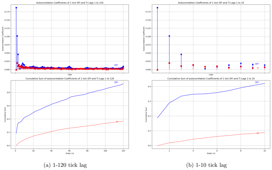
The central claim is that post-shock price dynamics are described by replacing the constant drift of geometric Brownian motion with an Ornstein-Uhlenbeck process driven by a zero-mean symmetric Lévy process with finite second moment: $\mathrm{d}S_t = \mu_t S_t\,\mathrm{d}t + \sigma S_t\,\mathrm{d}W_t$, $\mathrm{d}\mu_t = -\theta \mu_t\,\mathrm{d}t + \mathrm{d}L_t$, with initial drift $\mu_0 = OFI_0\,\rho_k$. Under this system the expected log-return is $\mathbb{E}[R_t] = \mu_0(1-e^{-\theta t})/\theta - \sigma^2 t/2$, the log-return variance is $\sigma^2 t + \frac{\sigma_L^2}{\theta^2}(t - \frac{2}{\theta}(1-e^{-\theta t}) + \frac{1}{2\theta}(1-e^{-2\theta t}))$, and their ratio defines a quasi-Sharpe ratio whose maximizing time is the optimal holding horizon. The paper reports that OFI-based LASSO regressions on CSI 300 index futures produce cumulative profits that saturate with forecast horizon in the shape the expected-return formula predicts, and that OFI keeps positive autocorrelation memory across regimes while weaker metrics change sign.
Load-bearing premise
The formulas stand on a linear signal-to-drift map, $\mu_0 = OFI_0\,\rho_k$, with a drift that reverts at constant speed $\theta$ and jump noise independent of price noise; if OFI impact is nonlinear, depth-dependent, or correlated with price noise, the closed-form mean, variance, and quasi-Sharpe ratio do not follow.
Editorial extensions
If this is right
- Expected returns after an OFI shock rise to a peak at $t = -(1/\theta)\ln(\sigma^2/(2\mu_0))$ and then decay, so each signal carries a finite optimal holding horizon.
- The quasi-Sharpe ratio has a finite-time maximum when the initial drift is large enough relative to volatility, defining a concrete execution time for OFI-based strategies.
- Horizon selection changes which companion metric helps: trade imbalance adds value at sub-second horizons and the cumulative OFI measure AvgEn adds value beyond two minutes, while OFI alone remains dominant across most horizons.
- A stable microstructure metric should keep positive autocorrelation memory and stable sign across market regimes; metrics such as raw mid-price changes that flip sign are weak standalone predictors.
- Near $t=0$ the model asymptotically matches constant-drift geometric Brownian motion, so the derived formulas are consistent with standard short-horizon behavior.
Reading between the lines
- The same three-formula structure could be applied to any signed microstructure signal with exponentially decaying autocorrelation, giving each signal its own $\theta$ and its own optimal holding time.
- The independence of $W_t$ and $L_t$ assumed in the variance derivation is testable: realized variance after large OFI shocks could be compared with equation (22), and the paper itself notes the two noises may be correlated.
- The monthly regime analysis suggests backtesting windows should be adapted to the current memory regime instead of extended arbitrarily, a practical rule the paper hints at but does not quantify.
- The predicted saturating return shape could be checked on other index futures or equities; a successful transfer would make the model a general screening device rather than a CSI 300-specific fit.
Editorial analysis
A structured set of objections, weighed in public.
Referee Report
Summary. The paper studies post-order-flow-imbalance price dynamics in CSI 300 index futures. It proposes a geometric Brownian motion model whose drift is an Ornstein-Uhlenbeck process driven by a symmetric Lévy process, motivated by stable contemporaneous OFI–price correlation and by the OU-like autocorrelation of OFI. The authors derive closed-form expressions for the log-return mean, variance, and a 'quasi-Sharpe ratio' (equations (20), (22), (24)), then conduct LASSO regressions across many historical windows and forecast horizons. They claim three findings: OFI acts as a mean-reverting jump-type shock; metric effectiveness is horizon-dependent; and OFI memory is regime-dependent across months.
Significance. If the model and derivations are correct, the paper offers a tractable continuous-time description of how an OFI shock propagates into expected returns and a risk-adjusted 'response ratio,' including a predicted optimal holding time. The appendices give explicit step-by-step derivations, which are useful and mostly standard. The empirical work is extensive in its grid over windows and horizons, and the out-of-sample LASSO split is a reasonable procedure. However, the significance is sharply reduced by three weaknesses: the variance/quasi-Sharpe results depend on an independence assumption the authors themselves question; the empirical validation is essentially visual and rests on very low R² values; and the risk-adjusted predictions are not empirically tested, as the paper acknowledges in Section 6.
major comments (5)
- [§2.4 and Appendix A.2] Equation (22) and therefore the quasi-Sharpe ratio (24) are derived under the assumption that the Lévy process Lt is independent of the Wiener process Wt. Section 2.4 immediately after system (14) states that Wt and Lt 'may exhibit correlation.' If Corr(L,W) is nonzero, the variance of the log-return acquires an additional cross-covariance term involving ∫(1−e^{-θ(t−u)})dL_u and σW_t, so (22) and (24) are not consequences of the model as stated. The paper neither estimates this correlation nor provides a sensitivity bound, yet the optimal holding time t* and the long-run equilibrium claims rest on (24). This is a load-bearing point for the risk-adjusted findings.
- [§3, Table B.1, Figure 3.1] The empirical validation is a visual comparison between LASSO PnL curves and 'model-predicted' curves, but the R² values in Table B.1 are extremely small (on the order of 0.004%–2%), and no standard errors, confidence intervals, or significance tests are given. Moreover, the model-predicted curves are not accompanied by an explicit calibration procedure for θ, ρ, k, and σ²; the paper does not report fitted parameter values or their uncertainties, nor does it test the quantitative predictions of (20) or the peak location predicted by the quasi-Sharpe ratio. The statement in Section 6 that variance validation is deferred implies that the central risk-adjusted predictions are untested.
- [§3.2 and Table B.1] The reported empirical total PnL increases monotonically with forecast horizon for essentially all historical window sizes (e.g., for historical window 1 tick, total PnL rises from 63,285 at 1 tick to 525,534 at 3600 ticks). This is inconsistent with the 'exponentially saturating then decaying' shape of E[R_t] in equation (20), which predicts a maximum followed by a decline as the −σ²t/2 term dominates. The paper's textual claim that the data exhibit 'similar patterns' to the model prediction is not supported by the numbers in Table B.1; the empirical curves appear to saturate rather than decay over the tested range.
- [§2.3–2.4] The mapping from OFI to the initial drift is specified as µ0 = OFI0 ρ k, where k is never defined. The contemporaneous correlation coefficient ρ is unitless, whereas OFI is measured in contracts or quantities and drift is in price units, so k is unidentified and dimensionally unspecified. The same issue appears in equation (12), where ρk multiplies the expected cumulative impact. Without a defined k or an estimated regression slope, the 'model-predicted' PnL curves in Figure 3.1(b) are not identifiable from the data, which weakens the claim that the empirical results validate the model.
- [§5] The section is titled 'regime-switching characteristics,' but no regime-switching model is estimated; the evidence consists of month-by-month autocorrelation coefficients. The claim that robust metrics show only 'quantitative' rather than 'qualitative' variation is asserted without a statistical test, and the proposed screening criteria in the conclusion are not formally validated out-of-sample. This weakens the third contribution stated in the abstract.
minor comments (9)
- [§2.3, Eq. (12)] Equation (12) contains a stray brace ('E[Sn}') and inconsistently uses n and t as the time index; it should be rewritten for clarity.
- [§2.3, Eq. (8)] The autocorrelation formula ρk = e^{−θkΔt} is derived for the continuous-time OU process, but equation (8) is a discrete-time difference equation; the paper should clarify the approximation and how Δt=1 is used to obtain ρk = (1−θ)^k.
- [§2.3] The paper states 'with our observed empirical autocorrelation decay rate θ = 0.5' without explaining how θ is estimated; given the substantial monthly variation in Table 5.1, a single θ=0.5 is not self-evident.
- [Appendix B] R² values are reported as percentages with many decimal places; consider reporting them as fractions or with a clear label, and consider adding a column for the number of observations.
- [§3.2] The claim of 'statistically significant improvements' in predictive coefficients is not backed by any significance test or confidence interval.
- [§1, references] The validation reference to Shen [2] is a PhD thesis; if used as external validation of Figure 2.5, the claim should be framed as unpublished or the paper should provide its own empirical counterpart.
- [Abstract and §2.4] The terms 'cost-effectiveness ratio,' 'quasi-Sharpe ratio,' and 'response ratio' are used interchangeably; a single term should be adopted throughout.
- [§3] The profitability results do not include transaction costs or market impact, which is important for the practical relevance of the PnL numbers.
- [Global] There are several typographical issues, including 'U-O process' (Section 1.2), 'Itˆo' (Section 2.3), and 'matrics' (Section 2.1).
Circularity Check
No circular derivation by construction; the SDE-to-formula results are self-contained, though the empirical confirmation is in-sample and the variance conclusion depends on an explicitly flagged independence assumption.
full rationale
The central derivation chain is not circular. The paper postulates an SDE system (14) in which the GBM drift follows a zero-mean OU process driven by a symmetric Lévy process, with initial drift µ0 = OFI0ρk. From this system, equations (20), (22), and (24) follow by direct stochastic calculus under stated assumptions; the mean and variance formulas are mathematical consequences of the model, not restatements of the data. The paper contains no load-bearing self-citations: reference [26] (Lehalle and Neuman) and [27,28] (Bel Hadj Ayed et al.) are external sources, and the OU/Lévy ansatz is explicitly argued from empirical autocorrelation and kurtosis rather than smuggled in via citation. The main weaknesses are non-circular. First, the empirical validation in Section 3.2 compares regression-based PnL curves to model-predicted curves generated using the same dataset to estimate θ and ρ, so the confirmation is in-sample consistency with fitted inputs rather than an independent out-of-sample prediction; this weakens the evidence but does not make the derivation equivalent to its inputs. Second, the variance formula (22) and the quasi-Sharpe conclusions depend on the independence of Wt and Lt, whereas Section 2.4 itself notes that Wt and Lt 'may exhibit correlation'; this is an unverified and potentially incorrect assumption, but it is an explicit assumption, not a circular step. Therefore, no specific circular reduction can be exhibited from the paper's own equations, and the appropriate finding is no significant circularity.
Assumptions & free parameters
free parameters (4)
- theta (mean-reversion speed θ) =
0.5 (approximate, inferred from halving autocorrelation of en)
- rho (correlation coefficient between OFI and mid-price changes) =
0.20 to 0.54 across windows (Table 2.1), used as ρk
- sigma_L^2 (per-unit-time variance of the Lévy process) =
not estimated; fixed at 0.04 in Figures 2.6-2.8
- sigma^2 (price volatility) =
not estimated; varied in model figures
assumptions (4)
- ad hoc to paper en and OFI follow an O-U process driven by a zero-mean symmetric Lévy process with finite second moment.
- domain assumption The Lévy process L_t and the Brownian motion W_t are independent.
- ad hoc to paper Price impact of OFI is linear in the drift: µ0 = OFI0ρk and dµt = -θµt dt + dLt.
- domain assumption The long-run mean of the OFI drift is zero (µl = 0).
Cite this review
Pith. "Pith review of Stochastic Price Dynamics in Response to Order Flow Imbalance: Evidence from CSI 300 Index Futures." pith.science (2026). https://pith.science/paper/R426ISA4
@misc{pith2026250517388,
  author       = {Pith},
  title        = {Pith review of: Stochastic Price Dynamics in Response to Order Flow Imbalance: Evidence from CSI 300 Index Futures},
  year         = {2026},
  howpublished = {\url{https://pith.science/paper/R426ISA4}},
  note         = {Machine review of arXiv:2505.17388}
}
read the original abstract
We conduct modeling of the price dynamics following order flow imbalance in market microstructure and apply the model to the analysis of Chinese CSI 300 Index Futures. There are three findings. The first is that the order flow imbalance is analogous to a shock to the market. Unlike the common practice of using Hawkes processes, we model the impact of order flow imbalance as an Ornstein-Uhlenbeck process with memory and mean-reverting characteristics driven by a jump-type L\'evy process. Motivated by the empirically stable correlation between order flow imbalance and contemporaneous price changes, we propose a modified asset price model where the drift term of canonical geometric Brownian motion is replaced by an Ornstein-Uhlenbeck process. We establish stochastic differential equations and derive the logarithmic return process along with its mean and variance processes under initial boundary conditions, and evolution of cost-effectiveness ratio with order flow imbalance as the trading trigger point, termed as the quasi-Sharpe ratio or response ratio. Secondly, our results demonstrate horizon-dependent heterogeneity in how conventional metrics interact with order flow imbalance. This underscores the critical role of forecast horizon selection for strategies. Thirdly, we identify regime-dependent dynamics in the memory and forecasting power of order flow imbalance. This taxonomy provides both a screening protocol for existing indicators and an ex-ante evaluation paradigm for novel metrics.
Figures


Figures from the paper (15 more)


Forward citations
Cited by 1 Pith paper
-
When Does Order Flow Matter? State-Dependent L2 Liquidity-State Transitions in Crypto Futures
In Binance BTC/ETH futures event windows, pre-event L2 liquidity state dominates post-event regime prediction; order flow helps only as an ETH-dominant, stress-amplified overlay.
Reference graph
Works this paper leans on
-
[1]
The price impact of order book events
Rama Cont, Arseniy Kukanov, and Sasha Stoikov. The price impact of order book events. Journal of Financial Econometrics, Vol. 12, No. 1, pp. 47–88, 2014
work page 2014
-
[2]
Order imbalance based strategy in high frequency trading
Darryl Shen. Order imbalance based strategy in high frequency trading. Ph.D. thesis, Oxford University, 2015
work page 2015
-
[3]
Cross-impact of order flow imbalance in equity markets
Rama Cont, Mihai Cucuringu, and Chao Zhang. Cross-impact of order flow imbalance in equity markets. Quantitative Finance, Vol 23, Issue 10, 2023
work page 2023
-
[4]
Price dynamics in a Markovian limit order market
Rama Cont and Adrien de Larrard. Price dynamics in a Markovian limit order market. SIAM Journal on Financial Mathematics, Vol. 4, No. 1, 2012
work page 2012
-
[5]
Order Book Dynamics in Liquid Markets: Limit Theorems and Diffusion Approximations
Rama Cont and Adrien de Larrard. Order Book Dynamics in Liquid Markets: Limit Theorems and Diffusion Approximations. SSRN Electronic Journal SSRN: https://ssrn.com/abstract=1757861, 2012
work page 2012
-
[6]
Optimal order placement in limit order markets
Rama Cont and Arseniy Kukanov. Optimal order placement in limit order markets. Quantitative Finance, Vol 17, Issue 1, pp.1-19, 2017
work page 2017
-
[7]
Rama Cont and Marvin S. Muller. A Stochastic Partial Differential Equation Model for Limit Order Book Dynamics. SIAM Journal on Financial Mathematics Vol. 12, Issue 2,2021
work page 2021
-
[8]
Koti S. Jaddu, Paul A. Bilokon. Combining Deep Learning on Order Books with Reinforcement Learning for Profitable Trading. SSRN Electronic Journal, ssrn.4611708, 2023
work page 2023
Show all 31 references
- [9]
-
[10]
How and when are high-frequency stock returns predictable? Available at SSRN 4095405, 2022
Yacine Ait-Sahalia, Jianqing Fan, Lirong Xue, and Yifeng Zhou. How and when are high-frequency stock returns predictable? Available at SSRN 4095405, 2022
2022
-
[11]
Asymmetric effects of the limit order book on price dynamics
Tolga Cenesizoglu, Georges Dionne, and Xiaozhou Zhou. Asymmetric effects of the limit order book on price dynamics. Journal of Empirical Finance, 65:77–98, 2022
2022
-
[12]
A characterisation of cross-impact kernels
Mathieu Rosenbaum and Mehdi Tomas. A characterisation of cross-impact kernels. arXiv preprint arXiv:2107.08684, 2021
2021 arXiv
-
[13]
A. G. Hawkes. Point spectra of some mutually exciting point processes. Journal of the Royal Statistical Society: Series B (Methodological), Vol. 33 , pp.438-443, 1971
1971
-
[14]
Optimal exercise of American options under time-dependent Ornstein–Uhlenbeck processes
Abel Azze, Bernardo D’Auria, Eduardo Garc ´ ıa-Portugu´ es. Optimal exercise of American options under time-dependent Ornstein–Uhlenbeck processes. Stochastics Vol 96, No.1, pp.921-946, 2024
2024
-
[15]
VIX pricing in the Bergomi model under a regime switching change of measure
Henrique Guerreiro, Jo˜ ao Guerra. VIX pricing in the Bergomi model under a regime switching change of measure. Quantitative Finance, Vol 23, No.5, pp.721-738, 2023
2023
-
[16]
A. H. Nzokem. Pricing European Options under Stochastic Volatility Models: Case of five-Parameter Variance-Gamma Process. Journal of Risk and Financial Management, Vol. 16, No.1, pp.55, 2023
2023
-
[17]
Bertram’s Pairs Trading Strategy with Bounded Risk.Central European Journal of Operations Research, Vol
Vladim ´ ır Hol´ y, MichalˇCern´ y. Bertram’s Pairs Trading Strategy with Bounded Risk.Central European Journal of Operations Research, Vol. 30, No. 2, pp.667-682, 2022
2022
-
[18]
Doyne Farmer, John Geanakoplos
Josep Perell´ o, Miquel Montero, Jaume Masoliver, J. Doyne Farmer, John Geanakoplos. Statistical analysis and stochastic interest rate modelling for valuing the future with implications in climate change mitigation. Stat. Mech. 043210, 2020
2020
-
[19]
Fast Pricing of Energy Derivatives with Mean-reverting Jump-diffusion Processes
Nicola Cufaro Petroni, Piergiacomo Sabino. Fast Pricing of Energy Derivatives with Mean-reverting Jump-diffusion Processes. Applied Mathematical Finance, 2021. 30
2021
-
[20]
Optimal Mean Reversion Trading with Transaction Costs and Stop-Loss Exit
Tim Leung, Xin Li. Optimal Mean Reversion Trading with Transaction Costs and Stop-Loss Exit. International Journal of Theoretical and Applied Finance, Vol. 18, No. 3, 2015
2015
-
[21]
Optimal closing of a pair trade with a model con- taining jumps
Stig Larsson, Carl Lindberg, Marcus Warfheimer. Optimal closing of a pair trade with a model con- taining jumps. Appl. Math. Vol. 58, pp.249-268, 2013
2013
-
[22]
Option pricing under Ornstein-Uhlenbeck stochastic volatility: a linear model
Giacomo Bormetti, Valentina Cazzola, Danilo Delpini. Option pricing under Ornstein-Uhlenbeck stochastic volatility: a linear model. Int. J. Theoretical Appl. Finance Vol.7 pp.1047-1063, 2010
2010
-
[23]
Probability distribution of returns in the exponential Ornstein-Uhlenbeck model
Giacomo Bormetti, Valentina Cazzola, Guido Montagna, Oreste Nicrosini. Probability distribution of returns in the exponential Ornstein-Uhlenbeck model. J. Stat. Mech. P11013, 2008
2008
-
[24]
Multi-asset optimal execution and statistical arbitrage strategies under Ornstein-Uhlenbeck dynamics
Philippe Bergault, Fay¸ cal Drissi, Olivier Gu´ eant. Multi-asset optimal execution and statistical arbitrage strategies under Ornstein-Uhlenbeck dynamics. arXiv:2103.13773
-
[25]
A closed-form solution for optimal mean-reverting trading strategies
Alexander Lipton, Marcos Lopez de Prado. A closed-form solution for optimal mean-reverting trading strategies. arXiv:2003.10502
2003 arXiv
-
[26]
Incorporating Signals into Optimal Trading
Charles-Albert Lehalle, Eyal Neuman. Incorporating Signals into Optimal Trading. Finance and Stochastics, Vol. 23, pp. 275–311, 2019
2019
-
[27]
Performance analysis of the optimal strategy under partial information
Ahmed Bel Hadj Ayed, Gr´ egoire Loeper, Sofiene El Aoud, Fr´ ed´ eric Abergel. Performance analysis of the optimal strategy under partial information. International Journal of Theoretical and Applied Finance, Vol. 20, No. 2, Oct 2015
2015
-
[28]
Forecasting trends with asset prices
Ahmed Bel Hadj Ayed, Gr´ egoire Loeper, Fr´ ed´ eric Abergel. Forecasting trends with asset prices. arXiv:1504.03934
-
[29]
Risk valuation of quanto derivatives on temperature and electricity
Aur´ elien Alfonsi, Nerea Vadillo. Risk valuation of quanto derivatives on temperature and electricity. Applied Mathematical Finance Vol. 30, No. 4, pp.1-38, 2024
2024
-
[30]
High-frequency trading: a practical guide to algorithmic strategies and trading systems, Second Edition, John Wiley, 2013
Irene Aldridge. High-frequency trading: a practical guide to algorithmic strategies and trading systems, Second Edition, John Wiley, 2013. ISBN-13: 978-1118343500
2013
-
[31]
µ0e−θt + Z t 0 e−θ(t−s)dLs 2# Expanding the expression, we have: E µ2 t = E
GE Uhlenback and LS Ornstein. On the theory of the brownian motion. Phys. Rev, 36:823–841, 1930. Appendix A Logarithmic return process derivations A.1 The variance of a certain O-U process A zero-mean-reverting Ornstein-Uhlenbeck (OU) process driven by a L´ evy process is desc...
1930
Reviewed August 7, 2026 · model on record in the stance chip above.
Discussion (0). Continue with ORCID to comment.