REVIEW 3 major objections 3 minor 40 references
Educational programs and crime: a compartmental model approach
T0 review · 3 major / 3 minor · reviewed 2026-08-07 · deepseek-v4-flash
Pith's one-line read The paper derives two thresholds, R0 and C, that fully determine whether a prison education program survives, dies out, or coexists with crime in a compartmental epidemic-like model.
desk verdict Solid theoretical extension of compartmental crime models with a clean threshold result; the empirical claims outrun the data and the X compartment mixes two populations, so the policy reading should be treated skeptically. read the letter →
The pith
A machine-rendered reading of the paper's core claim, the machinery that carries it, and where it could break.
The reading
What carries the argument
The machinery is a three-compartment ordinary differential equation system (X susceptible, I incarcerated non-students, E incarcerated students) with mass-action recruitment αXI and net educational flow ρ = φ − β from I to E. The next-generation matrix yields R0 = αΛ/(µ(γI+µ)), and the coexistence threshold C = 1 + α(γE+µ)/(ρ(γI+µ)) appears when the third eigenvalue at the education-free equilibrium changes sign. Theorem 2 uses the signs of R0 − 1 and R0 − C to decide which of the three equilibria is locally stable.
What would settle it
Track released prisoners and record how many re-offend before re-entering the non-offender pool; if that fraction is high, the model's I-to-X transition is wrong and neither R0 nor C would predict whether education programs survive. Equivalently, re-estimate R0 and C from the 1992–2024 Italian series with a state-space model that filters observation noise; if the inferred regime moves between education-free and coexistence across reasonable noise models, the threshold claim is not identifiable from current data.
Extended reading notes
Core claim
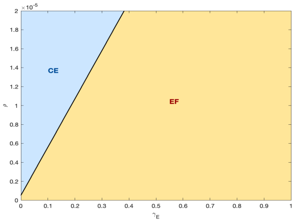
The central claim is that the asymptotic behavior of the crime-incarceration-education system is completely classified by R0 = αΛ/(µ(γI+µ)) and C = 1 + α(γE+µ)/(ρ(γI+µ)), with ρ = φ − β measuring the net flow into education. The delinquency-free equilibrium is locally stable when R0 < 1; the education-free equilibrium is locally stable when 1 < R0 < C; and the coexistence equilibrium is locally stable when R0 > C. The proof computes the eigenvalues of the Jacobian at each equilibrium, and the thresholds make explicit that educational parameters act only through C, never through R0. If the model is right, a prison education program survives only when the social transmission of crime is strong enough to pass a second, education-dependent threshold.
Load-bearing premise
The model's weakest load-bearing premise is that everyone outside prison is a single susceptible pool and that released inmates return to non-offending status; if most released prisoners re-offend quickly, the thresholds no longer describe reality.
Editorial extensions
If this is right
- Educational parameters do not appear in R0, so expanding prison education cannot by itself push crime below the extinction threshold; education acts only by changing C.
- Increasing the net enrollment rate ρ = φ − β or shortening the education-stay rate γE lowers C, so a fixed R0 > 1 can move the system from the education-free regime to coexistence.
- When R0 exceeds C, the approach to coexistence can be oscillatory (Corollary 4), so transient waves in prison and education populations are expected rather than signs of instability.
- The Italian data point estimate places the system at R0 ≈ 1.03 and C ≈ 1.10, predicting the education-free equilibrium, but the confidence interval for R0 crosses 1, so delinquency extinction cannot be ruled out from these data.
- Because R0 is independent of education, policy makers who want to eliminate delinquency entirely must act on the contact rate α, the release rate γI, or demographic flows, not on course offerings alone.
Reading between the lines
- Extension: because the X compartment includes offenders who have not yet been caught, the R0 estimated from prison counts is likely a lower bound on the true recruitment potential; splitting X into never-offenders and not-yet-incarcerated offenders would shift both thresholds.
- Extension: the model suggests an asymmetric policy lever—prison administrations can move a society from education-free to coexistence by increasing ρ, while lowering R0 requires broader criminal-justice and social changes, so coexistence may be the realistic near-term target.
- Testable extension: using post-2019 data on formal education levels (primary through university) rather than vocational completions could re-estimate C; if the regime shifts toward coexistence, that would support the model's qualitative prediction that stronger educational engagement lowers C.
- Extension: the damping rate of oscillations near the coexistence equilibrium is controlled by α(γE+µ)/(2ρ), so monitoring early oscillatory patterns in prison enrollment could provide an early warning of which regime the system is entering.
Signed reviews
Editorial analysis
A structured set of objections, weighed in public.
Referee Report
Summary. The paper presents a three-compartment ODE model (X susceptible, I incarcerated non-educated, E incarcerated educated) for crime as a social contagion. It derives three equilibria and uses the next-generation matrix to define R0 = αΛ/(µ(γI+µ)) and a threshold C = 1 + α(γE+µ)/(ρ(γI+µ)), proving in Theorem 2 that the delinquency-free equilibrium is stable if R0<1, the education-free equilibrium if 1<R0<C, and the coexistence equilibrium if R0>C. The paper also runs illustrative simulations and fits the discretized I-equation to Italian prison data (1992-2024) to estimate α and ρ, concluding that the system resides in the education-free regime.
Significance. The mathematical core is standard but competently executed: the next-generation computation and Jacobian stability analysis are internally consistent, and the simulations align with the theorem. The threshold structure provides a potentially useful policy taxonomy for when prison education can persist. However, the significance is limited by two problems: the X compartment conflates true susceptibles with non-incarcerated offenders, so the thresholds are not cleanly interpretable as crime-spread thresholds; and the empirical application uses an observable for E that does not match the model state, with confidence intervals that straddle the thresholds. These issues affect the central claim, hence major revision is needed.
major comments (3)
- [Section 2, Table 1 and first paragraph] The X compartment is defined both as "non-offenders" and as "offenders not currently in prison". These are different populations: one is susceptible to initiating offending, the other may already be active criminals. In system (1), the incidence term αIX uses X in both roles, so α conflates first-time offending with re-arrest or recidivism. Consequently R0 in Eq. (9) and C in Theorem 2 are not reproduction numbers for delinquent behavior; they quantify flows into prison from a mixed pool. The policy reading in the Introduction and Conclusion (whether a prison education program can survive) therefore does not follow from the mathematics. The authors should either restrict X to non-offenders and model recidivism explicitly, or justify why non-incarcerated offenders and true susceptibles have identical contact and transition rates.
- [Section 4.2, Eq. (14) and surrounding text] The empirical section sets X_k = N0 - I_k - E_k, so every non-incarcerated adult is treated as susceptible. Combined with the fitted I-equation, this reproduces the conflation of the previous major comment. Moreover, the observable for E is defined as the cumulative sum of inmates who completed vocational programs, while the model state E(t) is the current number of inmates enrolled in education. These are different quantities (a flow versus a stock), so the discretized equation (14) is not the forward-Euler version of the model's second ODE. The parameter estimates and the resulting R0 and C are therefore unreliable. The authors need to reconcile the observable with the state variable, for example by using enrollment counts or by explicitly modeling completion outflows.
- [Section 4.2, Eqs. (15)-(16) and Conclusion] The confidence interval for ρ, (-0.3347·10^-6, 0.4892·10^-6), includes zero and negative values, which violates the model's assumption ρ>0 stated in Section 2.1. The interval for R0, (0.9617, 1.0887), crosses both 1 and the estimated C = 1.0959. Thus the data do not determine which equilibrium regime applies, and the statement in the Conclusion that the system resides in the education-free equilibrium is not supported by the estimation. The authors should either impose ρ>0 in a constrained estimation and report the resulting regime probabilities, or explicitly conclude that the regime is undetermined from these data.
minor comments (3)
- [Throughout] The paper contains several typos, including "delinquence" (Abstract, Section 3), "interscctions" (Section 2.1), "threcshold" (Remark 3), and "reproductive" instead of "reproduction" in Section 3. These should be corrected.
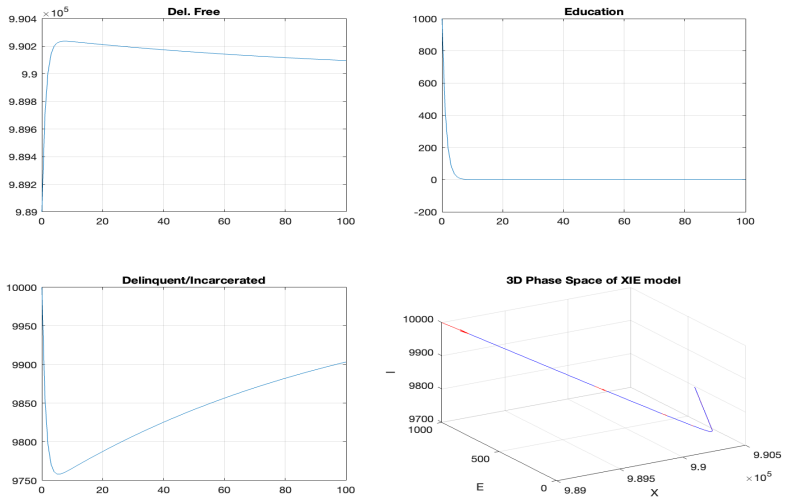
- [Section 4.1 and Figure 6] The text states that the education-free regime is obtained with γI = 0.985, while the caption of Figure 6 reports R0 = 1.01 and γI = 0.98. These values should be reconciled.
- [Section 2, I-compartment bullet] The assumption that released prisoners transition back to X and that re-offending is ignored "for a certain period whether minutes, hours, or days" is vague. Given that the time unit in simulations is a year and in the empirical part is a semester, this assumption needs a time-scale justification or a more precise statement of the intended interpretation.
Circularity Check
Empirical regime conclusion reduces to fitted parameters; theoretical stability derivation is self-contained.
-
fitted input called prediction
[Section 4.2, Eqs. (14)-(16) and the paragraph following Eq. (16)]
"Consequently, the parameters to be estimated are α and ρ. ... When discretized using the forward Euler method, this yields ... Ik+1 = Ik + αIk(N0 − Ik − Ek) − ρIkEk − γI Ik − µIk ... The optimal parameter values obtained using such a procedure are ˆα = 7.4037 · 10−9 ... ˆρ = 7.7230 · 10−8 ... The corresponding estimated value of the basic reproduction number is ˆR0 = 1.0252, while the threshold is estimated to be ˆC = 1.0959. In accordance with Theorem 2, these parameter estimates indicate a regime associated with the education-free equilibrium."
R0 and C are deterministic functions of the fitted parameters: R0 = αΛ/(µ(γI+µ)) and C = 1 + α(γE+µ)/(ρ(γI+µ)). The paper fits α and ρ by least squares to the I-compartment data using Eq. (14), then plugs those fitted values into R0 and C to conclude 1 < R0 < C, i.e. the education-free equilibrium. The regime statement is therefore a restatement of the fit, not an independent prediction. The comparison in Figure 9 is also in-sample: the trajectory is obtained by recursively applying the fitted equation (14) to the same data, so it provides no out-of-sample validation. The theoretical theorem is non-circular, but the empirical 'prediction' of the regime reduces by construction to the estimated parameters.
full rationale
The core mathematical content — the ODE system, the equilibria, the next-generation calculation of R0, and the Jacobian stability conditions in Theorem 2 — is derived directly from the stated model assumptions and is self-contained. No load-bearing self-citation, uniqueness import, or ansatz-smuggling via citation is present. The only circularity is in the empirical application: α and ρ are fitted from the I-equation data, and then R0 and C are computed from those same fitted values to classify the system's regime. Since R0 and C are defined as functions of α and ρ, the concluding statement that the system resides in the education-free equilibrium is forced by the fit. The paper does caution about the wide confidence intervals, and it frames the empirical part as an estimation/illustration rather than out-of-sample prediction, which is why the score is 6 rather than higher: the theoretical derivation remains independent, while one empirical conclusion is a fitted input renamed as a prediction.
Assumptions & free parameters
free parameters (2)
- alpha (contact/transmission rate) =
7.4037e-9 (95% CI: 0.0069e-6 to 0.0079e-6)
- rho (phi - beta, net education enrollment excess) =
7.7230e-8 (95% CI includes zero: -0.3347e-6 to 0.4892e-6)
assumptions (6)
- domain assumption Homogeneous mixing: all individuals have equal contact probability
- domain assumption Mass-action transmission for all transitions
- domain assumption Constant population N = Lambda/mu
- ad hoc to paper rho > 0 (phi > beta)
- domain assumption Released prisoners do not re-offend during the modeled period
- domain assumption The only pathway to crime is contact with offenders
Cite this review
Pith. "Pith review of Educational programs and crime: a compartmental model approach." pith.science (2026). https://pith.science/paper/BTH4TVMW
@misc{pith2026250517831,
  author       = {Pith},
  title        = {Pith review of: Educational programs and crime: a compartmental model approach},
  year         = {2026},
  howpublished = {\url{https://pith.science/paper/BTH4TVMW}},
  note         = {Machine review of arXiv:2505.17831}
}
abstract
In this paper, we present a mathematical model to describe the temporal evolution of delinquent behavior, treating it as a socially transmitted phenomenon influenced by peer interactions, thus similar to an epidemic. We consider a compartmental framework involving three ordinary differential equations to describe the dynamics among the three population groups: individuals not incarcerated (susceptible), incarcerated offenders, and incarcerated offenders participating in an educational program. Transitions between the groups are governed by interaction-based mechanisms that capture the influence of peer effects in the spread of criminal behavior. The model revealed three equilibrium states: a delinquence free equilibrium, an equilibrium where no criminals attend an educational program, and a coexistence equilibrium. The basic reproduction number, $R_0$, was derived, and a sensitivity analysis revealed the key parameters that influence the system's stability. The model thus provides a quantitative basis for evaluating the effectiveness of rehabilitation strategies in correctional settings. Numerical simulations and an empirical application illustrate the qualitative properties of the model and show how parameter variations influence system behavior.
Figures


Figures from the paper (6 more)




Reference graph
Works this paper leans on
-
[1]
Modeling dynamics of the spread of crime in a society
Srivastav AK, Ghosh M, Chandra P. Modeling dynamics of the spread of crime in a society. Stochastic Anal. Appl., 2019
work page 2019
-
[2]
Mathematical modeling of crime as a social epidemic
González-Parra G, Chen-Charpentier B, Kojouharov HV. Mathematical modeling of crime as a social epidemic. J Interdisc Math, doi: 10.1080/09720502.2015.1132574, 2018
-
[3]
Journal of Research in Crime and Delinquency 8: 124–132, 1971
Blumstein A, Larson RC Problems in modeling and measuring recidivism. Journal of Research in Crime and Delinquency 8: 124–132, 1971
work page 1971
-
[4]
Journal of Criminal Justice 1: 7–26, 1973
Belkin J, Blumstein A, Glass W Recidivism as a feedback process: An analytical model and empirical validation. Journal of Criminal Justice 1: 7–26, 1973
work page 1973
-
[5]
Blumstein A An OR missionary’s visits to the criminal justice system, Operations Research 55: 14–23, 2007
work page 2007
-
[6]
Blumstein A, Cohen J, Roth J, Visher CA Criminal Careers and Career Criminals. National Academy Press, 1986
work page 1986
-
[7]
Blumstein A, Cohen J,Characterizing criminal careers. Science 238: 985–991, 1982
work page 1982
-
[8]
Greenwood PW, Abrahamse A Selective incarceration. Rand Report R- 2815-NIJ, 1982
work page 1982
Show all 40 references
-
[9]
Criminology 35: 133–175, 1997
Canela-Cacho JA, Blumstein A, Cohen J Relationship between the offending frequency (λ) of imprisoned and free offenders. Criminology 35: 133–175, 1997
1997
-
[10]
Contributions to the mathematical theory of epi- demics
Kermack, W.O., McKendrick, A.G. Contributions to the mathematical theory of epi- demics. Bulletin of Mathematical Biology53 (1–2), 33–55, 1991. 24
1991
-
[11]
L., Franco, E., Mohler, G., Short, M
Bertozzi, A. L., Franco, E., Mohler, G., Short, M. B., Sledge, D. The challenges of modeling and forecasting the spread of COVID-19. Proceedings of the National Academy of Sciences, 117(29), 16732–16738, 2020
2020
-
[12]
Cerqueti, R., Ramponi, A., Scarlatti, S. A compartmental model for the dynamic simulation of pandemics with a multi-phase vaccination and its application to Italian COVID-19 data, Mathematics and Computers in Simulation, Volume 228, 124–146, ISSN 0378-4754, https://doi.org/10....
-
[13]
S., Wong, H
Chen, K., Pun, C. S., Wong, H. Y. Efficient social distancing during the COVID-19 pandemic: Integrating economic and public health considerations.European Journal of Operational Research, 304 (1), 84–98, 2022
2022
-
[14]
and Tessitore M.E
Ramponi A. and Tessitore M.E. (2023), The economic cost of social distancing during a pandemic: an optimal control approach in the SVIR model, Decision in Economics and Finance, 2023
2023
-
[15]
Gladwell, The Tipping Point: How Little Things Can Make A Big Difference, Little Brown and Company, Boston, 2000
M. Gladwell, The Tipping Point: How Little Things Can Make A Big Difference, Little Brown and Company, Boston, 2000
2000
-
[16]
Gino, Ayal S, Ariely D, Contagion and differentiation in unethical behavior, the effect of one bad apple on the barrel, Psychol
F. Gino, Ayal S, Ariely D, Contagion and differentiation in unethical behavior, the effect of one bad apple on the barrel, Psychol. Sci. 20, 393–398, 2009
2009
-
[17]
Lacey, M.N
A .A . Lacey, M.N. Tsardakas, A mathematical model of serious and minor criminal activity, Eur. J. Appl. Math. 27, 403–421, 2016
2016
-
[18]
Sooknanan, D.M.G
J. Sooknanan, D.M.G. Comissiong, When behaviour turns contagious: the use of de- terministic epidemiological models in modeling social contagion phenomena, Int. J. Dyn. Contr. 5 1046–1050, 2017
2017
-
[19]
D’Orsogna, M
M.R. D’Orsogna, M. Perc, Statistical physics of crime: a review, Phys. Life Rev. 1,2 1–21, 2015
2015
-
[20]
Sooknanan, B
J. Sooknanan, B. Bhatt, D.M.G. Comissiong, A modified predator-prey model for the interaction of police and gangs, R. Soc. Open Sci. 3, 2016
2016
-
[21]
Goyal, J
A. Goyal, J. Shukla, A. Misra, and A. Shukla. Modeling the role of government efforts in controlling extremism in a society. Mathematical Methods in the Applied Sciences, 2014
2014
-
[22]
McMillon, C
D. McMillon, C. P. Simon, and J. Morenoff. Modeling the underlying dynamics of the spread of crime. PLoS ONE, 9(4):e88923, 04 2014
2014
-
[23]
A. Misra. Modeling the effect of police deterrence on the prevalence of crime in the society. Applied Mathematics and Computation, 237:531–545, 2014. 25
2014
-
[24]
M. B. Short, P. J. Brantingham, and M. R. D’Orsogna. Cooperation and punishment in an adversarial game: How defectors pave the way to a peaceful society. Phys. Rev. E, 82:066114, 2010
2010
-
[25]
Cantrell, C
R. Cantrell, C. Cosner, and R. Manasevich. Global bifurcation of solutions for crime modeling equations. SIAM Journal on Mathematical Analysis, 44(3):1340?1358, 2012
2012
-
[26]
Manasevich, Q
R. Manasevich, Q. H. Phan, and P. Souplet. Global existence of solutions for a chemotaxis-typesystemarisingincrimemodelling.EuropeanJournalofAppliedMath- ematics, 24:273?296, 4, 2013
2013
-
[27]
Mohler and M
G. Mohler and M. Short. Geographic profiling from kinetic models of criminal behavior. SIAM Journal on Applied Mathematics, 72(1):163–180, 2012
2012
-
[28]
A. B. Pitcher. Adding police to a mathematical model of burglary. European Journal of Applied Mathematics, 21(4-5):401–419, 2010
2010
-
[29]
Rodriguez and A
N. Rodriguez and A. Bertozzi. Local existence and uniqueness of solutions to a pde model for criminal behavior. Mathematical Models and Methods in Applied Sciences, 20(supp01):1425–1457, 2010
2010
-
[30]
Short, A
M. Short, A. Bertozzi, and P. Brantingham. Nonlinear patterns in urban crime: Hotspots, bifurcations, and suppression. SIAM Journal on Applied Dynamical Sys- tems, 9(2):462–483, 2010
2010
-
[31]
M. B. Short, M. R. D’Orsogna, V. B. Pasour, G. E. Tita, P. J. Brantingham, A. L. Bertozzi, and L. B. Chayes. A statistical model of criminal behavior. Mathematical Models and Methods in Applied Sciences, 18(supp01):1249–1267, 2008
2008
-
[32]
J. B. Shukla, A. Goyal, K. Agrawal, H. Kuswah, and A. Shukla. Role of technology in combatingsocialcrimes: Amodelingstudy.EuropeanJournalofAppliedMathematics, 24:501–514, 8 2013
2013
-
[33]
W. Tao. Computational criminology and evolution mechanisms of social crime dynamic system. In Electronics, Computer and Applications, 2014 IEEE Workshop on, pages 481–484, May 2014
2014
-
[34]
Yokoyama and T
T. Yokoyama and T. Takahashi. Mathematical neurolaw of crime and punishment: The q-exponential punishment function. Applied Mathematics, 4, 1371–1375, 2013
2013
-
[35]
and Castillo-Chavez, C
Brauer, F. and Castillo-Chavez, C. Mathematical Models in Population Biology and Epidemiology. Springer Science, Berlin, 2010
2010
-
[36]
Kwofie, M
T. Kwofie, M. Dogbatsey, S.E. Moore Curtailing Crime Dynamics: A Mathematical Approach, Frontiers in Applied Mathematics and Statistics, 2023. 26
2023
-
[37]
60–69, 2018
Sooknanan J., Comissiong D.M.G., A mathematical model for the treatment of delin- quent behaviour, Socio–Economic Planning Sciences, v.63, pp. 60–69, 2018
2018
-
[38]
A dynamical mathematical model for crime evolution based on a compartmental system with interactions, International Journal of Computer Mathematics, 102(1), 44–59, 2024
Calatayud, J., Jornet, M., & Mateu, J. A dynamical mathematical model for crime evolution based on a compartmental system with interactions, International Journal of Computer Mathematics, 102(1), 44–59, 2024
2024
-
[39]
Calafiore, G.C., Novara, C., Possieri, C., A time-varying SIRD model for the COVID- 19 contagion in Italy, Annual Reviews in Control, 50, 361–372, 2020
2020
-
[40]
Complexity of the Basic Reproduction Number (R0)
Delamater PL, Street EJ, Leslie TF, Yang YT, Jacobsen KH. Complexity of the Basic Reproduction Number (R0). Emerg Infect Dis.,25(1):1-4. doi: 10.3201/eid2501.171901. PMID: 30560777; PMCID: PMC6302597, 2019. 27
2019 arXiv
Reviewed August 7, 2026 · model on record in the stance chip above.
Discussion (0). Continue with ORCID to comment.