REVIEW 3 major objections 6 minor 16 references
Beyond data: leveraging non-empirical information and expert knowledge in Bayesian model calibration
T0 review · 3 major / 6 minor · reviewed 2026-08-07 · deepseek-v4-flash
Pith's one-line read This paper claims that expert knowledge, scientific theory, and qualitative observations can be encoded as hard constraints in an approximate Bayesian target, so that models can be calibrated from knowledge alone or from knowledge plus…
desk verdict A useful, moderately novel ABC framework for imposing non-empirical constraints in calibration, with real potential for data-limited modeling; the main weaknesses are the hard-constraint treatment of expert knowledge and a few internal inconsistencies. read the letter →
The pith
A machine-rendered reading of the paper's core claim, the machinery that carries it, and where it could break.
The reading
What carries the argument
The load-bearing object is Equation (14), a target distribution that multiplies the prior by a likelihood for empirical data and by an indicator requiring the non-empirical discrepancy to vanish exactly: $$\pi(\$\theta$ \mid S_{\text{obs}}, y_{\text{obs}}) \propto \pi(\$\theta$)\, f(y_{\text{obs}} \mid \$\theta$) \int I\big(\rho(S_{\text{obs}}, S(y_{\text{sim}}(\$\theta$))) = 0\big)\, dy_{\text{sim}}.$$ Non-empirical statements are treated as directly observed summary statistics with range constraints (for example $S_{\text{obs}} \le a$), enforced by one-sided discrepancy functions such as $\rho = \max(b - a, 0)$ rather than the two-sided distances used in ordinary ABC, and acceptance requires zero discrepancy instead of a tolerance. A bespoke sequential Monte Carlo algorithm simultaneously anneals the likelihood and shrinks the discrepancy threshold to zero, which makes the combined target computationally feasible, and the same construction doubles as a simulation-based prior elicitation method because it automatically yields joint priors that respect parameter interdependencies.
What would settle it
Generate data from a known simulation model, then calibrate with an intentionally false expert constraint (for example, a recovery-time bound the generating dynamics violates) together with a large dataset; if the Equation (14) posterior concentrates on parameter values the data-only likelihood rules out, the zero-discrepancy assumption has demonstrably propagated expert error into the predictions.
Extended reading notes
Core claim
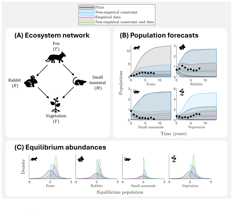
The paper's central claim is that anything we know about how a system behaves, such as an expert's bound on coral recovery, the theoretical requirement that all species coexist at a stable equilibrium, or the observation that a biochemical network must both respond to and adapt to stimulation, can be converted into a summary statistic plus a discrepancy function and enforced inside an approximate Bayesian target. When empirical data exist, a likelihood term multiplies the same target, producing a posterior that satisfies the data and the knowledge at once. The case studies show this is more than a formalism: data alone still admits coral trajectories that never recover, whereas data plus expert constraints match both sources; coexistence and stability constraints reverse the predicted effect of fox control on small mammals; and the efficient sampler finds adaptation-capable biochemical parameter sets outside the region the literature claimed was necessary.
Load-bearing premise
The framework treats every non-empirical statement as an exactly true constraint, requiring zero discrepancy, so if the expert knowledge is uncertain, biased, or poorly captured by the chosen summary statistics, the constrained posterior becomes overconfident and can be worse than ignoring the knowledge.
Editorial extensions
If this is right
- Models can be calibrated in the complete absence of empirical data, using only expert statements or qualitative observations, as in the coral growth and biochemical adaptation case studies.
- In sparse-data settings, adding non-empirical constraints eliminates predictions that conflict with established knowledge; the coral example shows that data alone still permits trajectories with virtually no recovery, which the constrained posterior rules out.
- Theory can change decisions: enforcing coexistence and stability in the ecosystem model reverses the predicted benefit of fox population control for small mammals.
- A more efficient search of the constrained parameter space can test claimed necessary conditions, since the biochemical case finds adaptation-capable parameter sets with $K_3 \ge 1$ or $K_4 \ge 1$, contrary to the conditions reported in the earlier literature.
- The framework provides a general simulation-based prior elicitation method that builds informed joint priors with parameter interdependencies captured automatically.
Reading between the lines
- A natural extension the paper does not build: treat expert statements as noisy constraints with a tolerance or error model, so uncertainty in the knowledge itself propagates into the posterior; the paper flags this need but leaves it as future work.
- A stress test the paper does not run: inject a deliberately wrong expert constraint alongside a rich dataset, and compare the constrained posterior with the data-only posterior to quantify how much overconfidence the exactness assumption can induce.
- The $K_3$/$K_4$ result hints that the sampler's efficiency could turn calibration into an auditing tool for other literature-derived necessary conditions in biology and ecology.
- Because empirical and non-empirical sources share one target, the framework could support sequential updating in which expert constraints are added, revised, or retracted as new data arrive.
Editorial analysis
A structured set of objections, weighed in public.
Referee Report
Summary. The paper proposes a Bayesian calibration framework that combines empirical data, modeled through a likelihood, with non-empirical information (expert knowledge, qualitative observations, scientific theory) encoded as ABC-style discrepancy constraints. The target distribution, Equation (14), multiplies the usual posterior by an indicator enforcing zero discrepancy for the non-empirical constraints. The authors develop an SMC algorithm that simultaneously anneals the likelihood and reduces the discrepancy threshold, and they demonstrate the approach on three case studies: logistic coral growth with expert recovery-time constraints, a four-species ecosystem model with coexistence/stability constraints plus time-series data, and a biochemical adaptation network with sensitivity/precision constraints. The paper claims this framework yields more realistic dynamics and more informed predictions than data-only calibration, and it also positions the method as a simulation-based prior elicitation tool.
Significance. If the central claims hold, the paper offers a coherent statistical way to fold non-empirical knowledge into model calibration, with broad applicability in ecology, biology, and medicine. The strengths include a clearly specified target distribution, a complete SMC algorithm, public code, and case studies that generate testable findings (e.g., the K3/K4 relationship in Case study 3). The simulation-based prior elicitation viewpoint is a useful contribution. However, the case studies are mostly synthetic demonstrations, and the hard-constraint formulation, which the paper itself acknowledges as a limitation in Discussion 3.3, is not accompanied by any sensitivity analysis or uncertainty quantification for the elicited constraints. This gap, together with internal numerical inconsistencies in Case study 3, tempers the strength of the main claims.
major comments (3)
- [§4.3, Eq. (14) and Discussion 3.3] The target distribution treats non-empirical statements as exact constraints via the indicator I(ρ=0). The paper acknowledges in Discussion 3.3 that elicited knowledge can contain uncertainties and biases, but it does not incorporate this uncertainty into the framework or test sensitivity to the chosen constraint thresholds. The case studies use hand-selected constraints (e.g., y(5)≤10%, y(50)≥K−1%, S>1, P>10) without demonstrating that nearby, equally plausible expert statements lead to similar posterior predictions. Since the central claim is that non-empirical information guides models toward more realistic dynamics, the missing load-bearing evidence is robustness to plausible variation in the non-empirical inputs.
- [Section 2.3.1 vs. Discussion 3.1] The reported sample size for the biochemical case study is internally inconsistent. Section 2.3.1 and Supplementary S.1.3 state that the SMC-ABC ensemble consists of 10,000 parameter sets, while Discussion 3.1 claims "we have obtained 10^5 parameter sets all of which are capable of adaptation." Additionally, Section 2.3 reports that Ma et al. (2009) found 1 in 10,000 (0.01%) adaptive parameterisations, whereas Discussion 3.1 says Ma et al. and Jeynes-Smith and Araujo (2023) tested 10^5 parameter sets with ~1% producing adaptation. These contradictions affect the paper's claims about computational efficiency and ensemble size and need to be resolved.
- [Sections 2.1 and 2.3] The demonstrations partly measure success by construction. The posterior is constrained to satisfy the non-empirical conditions, and then those same conditions are presented as the outcome (e.g., Figure 1B shows the posterior meets the recovery constraints; Figure 6E shows S>1 and P>10). The non-circular evidence is the management-prediction change in Section 2.2.2 (Figure 5) and the K3/K4 bivariate relationship in Section 2.3.2 (Figure 7), which are not restatements of the target constraints. To support the claim of "more realistic dynamics," the paper should either include an out-of-sample or additional-behavior validation or explicitly distinguish definitional success from independent predictive benefit.
minor comments (6)
- [Table S3 caption] The caption says "associated with the logistic growth model" but the table describes the ecosystem population model; it should refer to Section 2.2.
- [Section S.1.2 and Table S3] The text states that 16 parameters require calibration, but Table S3 lists 20 parameters (4 initial populations, 4 growth rates, 4 intra-specific interactions, 4 negative interactions, and 4 positive interactions); the count should be corrected.
- [Equation (13)] There is a typographical error in the exponent: the term should be (y_sim,i(θ)−y_obs,i)^2, and a closing parenthesis is missing in the display.
- [Discussion 3.1] The phrase "we have obtained 105 parameter sets" should read "10^5 parameter sets"; the superscript formatting appears to be lost.
- [Figure S6 caption] The caption contains a typo: "Michaelis-Mentin" should be "Michaelis-Menten."
- [Algorithm S1] The algorithm description should clarify that the target discrepancy threshold ε can be zero only for range-based constraints with a positive prior measure; for exact-value constraints, a tolerance would be needed, since a hard zero constraint on a continuous summary statistic generally has zero posterior mass.
Circularity Check
Demonstrations display the constraints encoded in the target as posterior behavior (self-definitional), but the central claims—management-prediction shifts and the K3/K4 finding—are not restatements of the inputs; score 3.
-
self definitional
[Section 2.1.1, Equations (3)-(7); Methods 4.3, Equation (14)]
"These two statements can be expressed in terms of the model parameters r, K and y0: ... y(5) <= 10% ... y(50) >= K-1% ... rho = rho5 + rho50 ... Models parameterised using both the prior and the non-empirical data sources exhibit the two desired behaviours: slow initial growth and recovery at 50 years."
Equation (14) defines the posterior as proportional to pi(theta) f(y_obs|theta) I(rho=0), and Equations (5)-(7) define rho so that rho=0 exactly when y(5)<=10 and y(50)>=K-1. Therefore every accepted posterior parameter set must satisfy the two expert constraints. Showing that posterior forecasts exhibit slow initial growth and 50-year recovery is not an independent empirical outcome; it is a restatement of the acceptance condition used to define the posterior. The independent content in this case study is the parameter-interdependency analysis (Figure 2) and the comparison with the data-only posterior (Figure 3), not the constraint-satisfaction display itself.
-
self definitional
[Section 2.2, Equation (8); Methods 4.3, Equation (14)]
"All eight summary statistics ... are combined within a single discrepancy function rho, calculated as rho = sum |min{0, n*_i}| + sum |max{0, R(lambda_j)}|, where rho measures the discrepancy in equilibrium behaviour from the theorised coexisting and stable behaviour ... The long-term non-empirical constraints are required to ensure that the system's equilibrium matches the ecological theory (Figure 4C, blue; Figure S5)."
By construction, rho=0 in Equation (8) if and only if all equilibrium abundances are positive and all real parts of the Jacobian eigenvalues are negative. Equation (14) targets exactly I(rho=0), so the equilibrium-constrained posterior is forced to contain only feasible, stable parameter sets. Displaying positive equilibria and negative eigenvalue real parts (Figure 4C, Figure S5) is therefore the definition of the posterior, not a discovered property. The genuinely non-circular result is the management-scenario difference in Figure 5, which is not directly encoded in the non-empirical constraint.
1 more flagged steps
-
self definitional
[Section 2.3, Equation (11); Section 2.3.1, Figure 6C/E]
"Hence, we can utilise these two summary statistics (sensitivity and precision) to define a measure of discrepancy rho between adaptive biochemical networks and a model simulation as rho = max(0,1-S) + max(0,10-P) ... simulations from the posterior show the output is both sensitive to stimulation and precisely able to return to pre-stimulation levels."
The discrepancy function in Equation (11) equals zero precisely when S>=1 and P>=10, which are the paper's definitions of sensitivity and precision. Sampling from the posterior defined by Equation (14) with I(rho=0) therefore guarantees that the sampled parameter sets are adaptation-capable. The posterior traces in Figure 6C/E showing sensitive and precise responses are a direct consequence of the acceptance condition, not an independent validation. The non-circular contribution is the bivariate K3/K4 finding in Figure 7, which emerges from the sampled ensemble rather than being imposed by rho.
full rationale
The central statistical construction, Equation (14), is a posterior conditioned on non-empirical constraints via the hard indicator I(rho=0). Because each case-study discrepancy function is deliberately built so that rho=0 encodes the expert statement, the displays showing that constrained posteriors satisfy those statements reduce to the definition of the target distribution. Those displays are therefore self-definitional rather than empirical evidence. However, the paper's main contributions do not rest on those displays alone: the data-only versus constrained-posterior comparison (Figure 3), the management-prediction shift under fox control (Figure 5), and the K3/K4 bivariate relationship (Figure 7) are not encoded in the constraints and provide independent content. The self-citations to Vollert et al. (2024, 2025) and Drovandi and Pettitt (2011) are used as standard ABC/SMC machinery; no uniqueness theorem is imported from the authors and no fitted parameter is relabeled as a prediction. The acknowledgment in Discussion 3.3 that the method treats non-empirical information as 'generally irrefutable' identifies a robustness/overconfidence limitation, but that is a correctness risk rather than a circularity. Overall, the circularity is partial and confined to the illustrative 'posterior satisfies its own constraints' demonstrations, so the score is 3 rather than higher.
Assumptions & free parameters
free parameters (3)
- Hand-chosen prior bounds in case studies =
various uniform/log-uniform ranges (e.g., r~U(0,0.5), K~U(60,80), log rates~U(-3,4))
- Non-empirical constraint thresholds =
10% at 5 yr; 1% of K at 50 yr; S>1; P>10; feasible and stable equilibrium
- SMC tuning parameters =
a=0.6, ESS_min=0.3, c=0.99, n_MCMC=10
assumptions (5)
- domain assumption The discrepancy function and chosen summary statistics fully capture the relevant non-empirical knowledge.
- ad hoc to paper Non-empirical information should be enforced with zero tolerance as an exact constraint.
- domain assumption The ODE models are sufficiently faithful simulators.
- standard math ABC with an indicator kernel is an acceptable likelihood approximation in this setting.
- domain assumption The synthetic datasets are representative of realistic sparse observations.
Cite this review
Pith. "Pith review of Beyond data: leveraging non-empirical information and expert knowledge in Bayesian model calibration." pith.science (2026). https://pith.science/paper/BM3OQETF
@misc{pith2026250521934,
  author       = {Pith},
  title        = {Pith review of: Beyond data: leveraging non-empirical information and expert knowledge in Bayesian model calibration},
  year         = {2026},
  howpublished = {\url{https://pith.science/paper/BM3OQETF}},
  note         = {Machine review of arXiv:2505.21934}
}
read the original abstract
Mathematical models connect theory with the real world through data, enabling us to interpret, understand, and predict complex phenomena. However, scientific knowledge often extends beyond what can be empirically measured, offering valuable insights into complex and uncertain systems. Here, we introduce a statistical framework for calibrating mathematical models using non-empirical information. Through examples in ecology, biology, and medicine, we demonstrate how expert knowledge, scientific theory, and qualitative observations can meaningfully constrain models. In each case, these non-empirical insights guide models toward more realistic dynamics and more informed predictions than empirical data alone could achieve. Now, our understanding of the systems represented by mathematical models is not limited by the data that can be obtained; they instead sit at the edge of scientific understanding.
Figures


Figures from the paper (4 more)


Reference graph
Works this paper leans on
-
[1]
Adams, M. P., S. A. Sisson, K. J. Helmstedt, C. M. Baker, M. H. Holden, M. Plein, J. Hol- loway, K. L. Mengersen, and E. McDonald-Madden (2020). Informing management deci- sions for ecological networks, using dynamic models calibrated to noisy time-series data. Ecology Letters 23(4), 607–619. 9, 10, 11 Allesina, S. and S. Tang (2012). Stability criteria f...
work page 2020
-
[2]
Springer. 2 Bhagowati, B. and K. U. Ahamad (2019). A review on lake eutrophication dynamics and recent developments in lake modeling.Ecohydrology & Hydrobiology 19(1), 155–166. 4 Bhattacharya, P., K. Raman, and A. K. Tangirala (2023). On biological networks capable of robust adaptation in the presence of uncertainties: A linear systems-theoretic approach....
work page 2019
-
[4]
These Michaelis constants are calculated using the association, dissociation and catalytic rates as Ki = (di +k i)/ai,(S33) whereK i is theith Michaelis-Menten constant. Previous literature indicates that for this biochemical network to be capable of adaptation, bothK 3 <1 andK 4 <1 (Ma et al., 2009; Jeynes-Smith and Araujo, 2023). 35 S.2 Additional resul...
work page 2009
-
[10]
For more information on this model and its parameters, see Jeynes-Smith and Araujo (2023)
All 12 parameters in the model are highly uncertain and require calibration (see Table S5). For more information on this model and its parameters, see Jeynes-Smith and Araujo (2023). Parameter Description Prior ai fori={1,2,3,4} Association rates logai ∼ U(−3,4) di fori={1,2,3,4} Dissociation rates logdi ∼ U(−3,4) ki fori={1,2,3,4} Catalytic rates logki ∼...
work page 2023
-
[14]
34 Initial condition Value A(0) 10 A∗(0) 0 B(0) 10 B∗(0) 0 E1(0) 1 E4(0) 1 C1(0) 0 C2(0) 0 C3(0) 0 C4(0) 0 Table S6: Initial condition parameter values assumed in the biochemical network model used in Section 2.3, Case study 3: Biochemical adaptation. For the system to be considered adaptive, two conditions must be met after it is stimulated: sensitivitya...
work page 2009
-
[16]
19 Graham, N., K. Nash, and J. Kool (2011). Coral reef recovery dynamics in a changing world. Coral Reefs 30, 283–294. 16 Grilli, J., M. Adorisio, S. Suweis, G. Barab´ as, J. R. Banavar, S. Allesina, and A. Maritan (2017). Feasibility and coexistence of large ecological communities.Nature Communica- tions 8(1), 1–8. 9, 10, 32 Harper, A., N. Mustafee, and ...
work page 2011
-
[17]
3, 4, 10, 17 Warne, D. J., K. Crossman, G. E. Heron, J. A. Sharp, W. Jin, P. P.-Y. Wu, M. J. Simpson, K. Mengersen, and J.-C. Ortiz (2024). Mathematical modelling and uncertainty quantifica- tion for analysis of biphasic coral reef recovery patterns.arXiv preprint arXiv:2406.19591. 16 Warne, D. J., K. A. Crossman, W. Jin, K. Mengersen, K. Osborne, M. J. S...
work page Pith review arXiv 2024
-
[27]
2 Rachel, L. (2024). The second wave.Review of Economic Design. 4 27 Raymond, B., J. McInnes, J. M. Dambacher, S. Way, and D. M. Bergstrom (2011). Qualita- tive modelling of invasive species eradication on subantarctic Macquarie Island.Journal of Applied Ecology 48(1), 181–191. 17 Rendall, A. R., D. R. Sutherland, C. M. Baker, B. Raymond, R. Cooke, and J....
work page 2024
Show all 16 references
-
[78]
Scott Mills, J
2 Humbert, J.-Y., L. Scott Mills, J. S. Horne, and B. Dennis (2009). A better way to estimate population trends.Oikos 118(12), 1940–1946. 17 Jakeman, A. J., R. A. Letcher, and J. P. Norton (2006). Ten iterative steps in development and evaluation of environmental models.Enviro...
2009
-
[204]
4 Gamerman, D. and H. F. Lopes (2006).Markov chain Monte Carlo: Stochastic simulation for Bayesian inference. CRC Press. 19, 40 Geary, W. L., M. Bode, T. S. Doherty, E. A. Fulton, D. G. Nimmo, A. I. Tulloch, V. J. Tulloch, and E. G. Ritchie (2020). A guide to ecosystem models ...
2006
-
[233]
3, 7, 22, 35, 41 Fava, M. C., N. Abe, C. Restrepo-Estrada, B. Y. Kimura, and E. M. Mendiondo (2019). Flood modelling using synthesised citizen science urban streamflow observations.Journal of Flood Risk Management 12(S2), e12498. 4 Felce, D. and J. Perry (1995). Quality of lif...
2019
-
[241]
2 Lundby, C. and P. Robach (2015). Performance enhancement: what are the physiological limits?Physiology. 4 Ma, W., A. Trusina, H. El-Samad, W. A. Lim, and C. Tang (2009). Defining network topologies that can achieve biochemical adaptation.Cell 138(4), 760–773. 13, 14, 16, 17,...
2015
-
[555]
3 Girolami, M. (2008). Bayesian inference for differential equations.Theoretical Computer Science 408, 4 –
2008
-
[1757]
13 Araujo, R. P. and L. A. Liotta (2023). Only a topological method can identify all possi- ble network structures capable of robust perfect adaptation.PLoS Computational Biol- ogy 19(11), e1011638. 13 Assump¸ c˜ ao, T. H., I. Popescu, A. Jonoski, and D. P. Solomatine (2018). ...
2023
-
[2006]
or the approximate posterior distribution (Sisson et al., 2007). SMC is a generally reliable sampling algorithm, and in particular, it is robust to the shape of the target distribution, minimises convergence issues, and is efficient when acceptance rates are low or the number ...
2007
-
[2012]
and is measured by taking the eigenvaluesλof the Jacobian matrixJevaluated at equilibriumn ∗. For Lotka-Volterra each element (i, j) of the Jacobian Jis calculated asJ i,j =α i,jn∗ i ,∀i, jin{F, R, M, V}such that the summary statistics for stability are real components of the ...
2024
Reviewed August 7, 2026 · model on record in the stance chip above.
Discussion (0). Sign in to comment.