REVIEW 2 major objections 4 minor 1 cited by
Dynamic State-Feedback Control for LPV Systems: Ensuring Stability and LQR Performance
T0 review · 2 major / 4 minor · reviewed 2026-08-07 · deepseek-v4-flash
Pith's one-line read The paper claims that a projected-gradient-flow controller can stabilize polytopic LPV systems with constant input matrix under arbitrarily fast parameter variations while converging to the LQR-optimal feedback gain for constant parameter…
desk verdict A useful new combination of projected gradient flow and LPV stability, but the advertised LQR-optimality result rests on an assumption that can be infeasible, and the frozen-time stability proof has a genuine gap. read the letter →
The pith
A machine-rendered reading of the paper's core claim, the machinery that carries it, and where it could break.
The reading
What carries the argument
The load-bearing mechanism is the projected gradient flow on a hyperrectangle C. The LQR cost f_K(ρ) = tr(P_K) has gradient ∇f_K = 2(RK − B^T P_K)Y_K, and the controller replaces this gradient by its projection onto the tangent cone of C using the projection matrix M(K) = I − J_g^T $F^{{-1}}$ J_g; the projection keeps vec(K) inside int(C), keeping the gradient well-defined and the controller trajectories bounded. The second mechanism is the polytopic reinterpretation: treating vec(K) as an extra parameter turns the state subsystem into a polytopic LPV system over P × C with N = |vert(P)| · $2^{{mn}}$ vertices, so quadratic stability becomes the finite LMI condition (27).
What would settle it
Compute the quantities d_i of Proposition 5 for a candidate system; if any d_i = 0, or if the range of optimal gains K*_ρ exits the interior of K_P, then no such box C exists and the controller's stability and convergence guarantees cannot be met.
Extended reading notes
Core claim
The central claim is that the controller defined by the projected gradient flow of the frozen-time LQR cost achieves two objectives simultaneously under Assumption 3. First, with the controller gain confined to the hyperrectangle C, the state subsystem can be reinterpreted as a polytopic LPV system in the augmented parameter (ρ, vec K), so quadratic stability is equivalent to a finite set of vertex LMIs; this gives exponential stability for all piecewise-continuous parameter trajectories. Second, for a constant parameter ρ, the projected flow has a single stationary point inside C, namely the LQR-optimal gain K*_ρ, and the flow converges to it. The paper further shows that the full closed-loop equilibrium (0, K*_ρ) is asymptotically stable, with region of attraction R^n × int(C).
Load-bearing premise
The results hold only if there exists a rectangular box of feedback gains that contains every LQR-optimal gain for all parameter values and is itself entirely contained in the set of gains stabilizing all frozen parameter systems; the paper gives no constructive test for when such a box exists.
Editorial extensions
If this is right
- For any system satisfying Assumption 3, fast parameter variation does not force a choice between stability and LQR performance: the same controller yields quadratic stability for all piecewise-continuous trajectories and converges to the optimal gain when the parameter freezes.
- The quadratic-stability certificate is a finite LMI feasibility problem over N = |vert(P)| · 2^{mn} vertices, so it can be checked with standard convex solvers.
- For constant parameter trajectories, the closed-loop equilibrium (0, K*_ρ) is asymptotically stable and its domain of attraction contains R^n × int(C), meaning any initial state can be used as long as the initial gain lies inside C.
- With piecewise-constant parameter trajectories and a sufficiently large learning rate, the controller spends most time operating at the LQR-optimal gain, which improves transient performance relative to a fixed feedback gain.
- Under slow parameter variation, the frozen-time asymptotic stability established in Theorem 4 combines with rate bounds to give exponential stability, with the admissible rate of gain variation controlled by the learning rate α.
Reading between the lines
- Editorial inference: the hard step is finding the box C; because the paper checks C ⊆ K_P through nonconvex distance problems and over-approximates K* through nonconvex CARE-constrained optimization, a practical rollout of the method would need tractable relaxations or a constructive search over C.
- Editorial inference: for quasi-LPV systems where ρ depends on the state, the augmented-polytope argument breaks down because K(t) and x(t) no longer enter as independent parameters; one testable extension would be to add a bound on ˙ρ and use the slow-variation conditions instead.
- Editorial inference: the simulation compares only against one fixed gain; a dynamic gain-scheduled benchmark that switches to K*_ρ instantly would clarify how much of the reported 26 percent cost reduction comes from adaptation rather than from the particular fixed comparison point.
Editorial analysis
A structured set of objections, weighed in public.
Referee Report
Summary. The paper proposes a dynamic state-feedback controller for polytopic LPV systems with a constant input matrix. The controller gain is updated by a projected gradient flow of the LQR cost, constrained to a hyperrectangle C in gain space. The paper derives a convex LMI condition (Theorem 2) for quadratic stability of the state subsystem when the gain trajectory stays in C, and gives sufficient conditions (Propositions 4–6 and Assumption 3) for boundedness of the gain trajectory and for its convergence to the optimal frozen-time LQR gains. Theorems 4 and 5 claim asymptotic stability of the closed-loop equilibrium for constant parameter trajectories, and a simulation example illustrates improved transient performance.
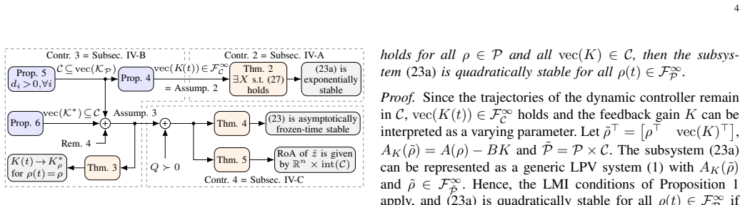
Significance. The idea of an online adaptive feedback gain that is projected onto a set of stabilizing gains is interesting and potentially useful for LPV systems. The quadratic stability certificate of Theorem 2 is convex and the dependency diagram in Fig. 1 is a helpful structural aid. The convergence claim for constant parameter trajectories is a non-circular application of existing policy-gradient results rather than a fitted or self-referential argument. However, the closed-loop stability theorem contains an invalid proof step, and the key Assumption 3 is not accompanied by any existence or applicability characterization. Because these issues affect the central claims, the paper needs substantial revision before it can be accepted.
major comments (2)
- [§IV-C, proof of Theorem 4 (Eqs. (39)–(41))] The proof concludes that ̇P_K ≺ 0 from tr(̇P_K) < 0. This implication is invalid: a symmetric matrix can have negative trace without being negative definite. Since Eq. (39) contains the term x^⊤ ̇P_K x, the negativity of ̇f_K alone does not control this term, and the claimed inequality ̇V < 0 is not established. The same gap affects Theorem 5, whose proof relies on the same strict decrease of V. The authors should either provide a valid argument for ̇P_K ≺ 0 (or prove ̇V < 0 by a different decomposition), or weaken the statement accordingly.
- [§IV-B, Assumption 3 and Propositions 5–6] Assumption 3 is the linchpin of Theorems 3–5, yet the paper provides no existence result or constructive characterization of systems for which such a hyperrectangle C exists. The verification route in Propositions 5 and 6 and Remark 3 relies on nonconvex global optimization problems (31) and (34) and requires unique global solutions, which are not guaranteed. Moreover, Assumption 3 does not follow from Assumption 1. For the scalar system ẋ = ρx + u with ρ ∈ [0,2] and Q = R = 1, one has K*_0 = 1 while K_P = {K ∈ R : K > 2}, so no interval C can contain vec(K*) and be contained in vec(K_P). The paper should either prove existence under checkable conditions or explicitly delimit the class of admissible systems, and it should discuss this example.
minor comments (4)
- [§II-C] The sentence 'The optimization problem (12) can be locally solved using (21)' appears to refer to equation (16), not (21).
- [§IV-B, proof of Lemma 4] The assertion that J_g^⊤v = 0 implies v = 0 because J_g^⊤ has full row rank is false when l > n; the null space has dimension l − n. The lemma's statement may still be correct for the hyperrectangle constraints, but the proof as written needs to be corrected.
- [§I-C] 'This section continuous with notation' should read 'continues with notation'.
- [§V] The text refers to 'Proposition (5)' where it should say 'Proposition 5', and the sentence 'For the solid lines, the switch occurs after convergence to K*_2 and K*_0.5 is reached' is confusingly worded.
Circularity Check
No significant circularity: the paper's stability and LQR-convergence results are conditional theorems built on external gradient-flow and LMI results, with no fitted parameter renamed as a prediction.
full rationale
The derivation chain is not circular. The dynamic controller (20) is defined directly as a projected policy gradient flow, and its convergence to the optimal LQR gain for constant rho (Theorem 3) is inherited from the external single-stationary-point analysis of [23] and the projection-flow theory of [25], neither of which is authored by the present paper's authors. The quadratic-stability condition (Theorem 2) is obtained by interpreting the constrained controller state as an additional parameter and applying the standard polytopic LPV vertex LMI (Theorem 1), so the verification LMI (27) is not assumed equivalent to the conclusion but is a genuine sufficient condition. The containment Assumption 3 (vec(K*) subset int(C) and C subset vec(K_P)) is an explicit sufficient condition, not a hidden fit; the hyperrectangle C is computed beforehand from CARE solutions via Proposition 6, and the later convergence claim is not used to define C. No data-fitting or self-referential prediction appears anywhere. Concerns about the possible infeasibility or conservativeness of Assumption 3 are scope and applicability limitations, not circular reasoning, because they do not make the theorem's conclusion coincide with its premises by construction.
Assumptions & free parameters
free parameters (2)
- learning rate alpha =
alpha = 100 in simulation; alpha > 0 in theory
- hyperrectangle C (2mn bounds) =
Simulation: C = [-0.94, -0.23] x [4.49, 5.97]
assumptions (4)
- domain assumption Assumption 1: (A(rho), B) is stabilizable and (A(rho), sqrt(Q)) is detectable for all rho in P; Q is positive semidefinite and R is positive definite.
- ad hoc to paper Assumption 3: there exists a hyperrectangle C with vec(K*) in int(C) and C subset vec(K_P), and K(0) is in int(C).
- ad hoc to paper Unique global solutions of the nonconvex optimization problems (31) and (34) can be obtained.
- standard math External results from [23] (single stationary point and gradient flow convergence), [25] (projected gradient flow properties), and [26, Th. 11.2.1] (continuity of the CARE solution) hold as cited.
Cite this review
Pith. "Pith review of Dynamic State-Feedback Control for LPV Systems: Ensuring Stability and LQR Performance." pith.science (2026). https://pith.science/paper/2QYQQYMQ
@misc{pith2026250522248,
  author       = {Pith},
  title        = {Pith review of: Dynamic State-Feedback Control for LPV Systems: Ensuring Stability and LQR Performance},
  year         = {2026},
  howpublished = {\url{https://pith.science/paper/2QYQQYMQ}},
  note         = {Machine review of arXiv:2505.22248}
}
read the original abstract
In this paper, we propose a novel dynamic state-feedback controller for polytopic linear parameter-varying (LPV) systems with constant input matrix. The controller employs a projected gradient flow method to continuously improve its control law and, under established conditions, converges to the optimal feedback gain of the corresponding linear quadratic regulator (LQR) problem associated with constant parameter trajectories. We derive conditions for quadratic stability, which can be verified via convex optimization, to ensure exponential stability of the LPV system even under arbitrarily fast parameter variations. Additionally, we provide sufficient conditions to guarantee the boundedness of the trajectories of the dynamic controller for any parameter trajectory and the convergence of its feedback gains to the optimal LQR gains for constant parameter trajectories. Furthermore, we show that the closed-loop system is asymptotically stable for constant parameter trajectories under these conditions. Simulation results demonstrate that the controller maintains stability and improves transient performance.
Figures


Figures from the paper (1 more)

Forward citations
Cited by 1 Pith paper
-
Hidden Star-Convexity in Policy Optimization for Gain-Scheduled LQR: Extended Version
For gain-scheduled LQR, the cost is exactly star-convex about the optimum under a covariance-substituted gradient, and a single mismatch ratio below one certifies linear convergence of gradient descent.
Reference graph
Works this paper leans on
-
[23]
J. Bu, A. Mesbahi, and M. Mesbahi, Policy Gradient-based Algorithms for Continuous-time Linear Quadratic Control ,
-
[25]
Constrained global optimization: Adaptive gradient flows,
H. T. Jongen and O. Stein, “Constrained global optimization: Adaptive gradient flows,” in Frontiers in Global Optimization, Springer, 2003
work page 2003
-
[1]
C. Hoffmann and H. Werner, “A survey of linear parameter- varying control applications validated by experiments or high- fidelity simulations,” IEEE Transactions on Control Systems Technology, no. 2, 2015
work page 2015
-
[2]
J. Mohammadpour and C. W. Scherer, Eds., Control of Linear Parameter Varying Systems with Applications , Springer Sci- ence & Business Media, 2012
work page 2012
-
[3]
C. Briat, Linear Parameter-Varying and Time-Delay Systems: Analysis, Observation, Filtering & Control (Advances in De- lays and Dynamics). Springer, 2015
work page 2015
-
[4]
Survey of gain-scheduling analysis and design,
D. J. Leith and W. E. Leithead, “Survey of gain-scheduling analysis and design,” Int. J. Control , no. 11, 2000
work page 2000
-
[5]
Analysis and design of gain scheduled control systems,
J. S. Shamma, “Analysis and design of gain scheduled control systems,” Ph.D. dissertation, MIT, 1988
work page 1988
-
[6]
Gain scheduling: Potential haz- ards and possible remedies,
J. Shamma and M. Athans, “Gain scheduling: Potential haz- ards and possible remedies,” IEEE Control Systems Magazine, no. 3, 1992
work page 1992
Show all 30 references
-
[7]
Control of linear parameter varying systems,
F. Wu, “Control of linear parameter varying systems,” Ph.D. dissertation, University of California, Berkeley, 1995
1995
-
[8]
Sufficient conditions for stability of linear time-varying systems,
A. Ilchmann, D. Owens, and D. Pr ¨atzel-Wolters, “Sufficient conditions for stability of linear time-varying systems,” Sys- tems & Control Letters , no. 2, 1987
1987
-
[9]
A. P. White, G. Zhu, and J. Choi, Linear Parameter-Varying Control for Engineering Applications (SpringerBriefs in Elec- trical and Computer Engineering). 2013
2013
-
[10]
Research on gain scheduling,
W. J. Rugh and J. S. Shamma, “Research on gain scheduling,” Automatica, no. 10, 2000
2000
-
[11]
Induced L2-norm control for LPV systems with bounded parameter variation rates,
F. Wu et al., “Induced L2-norm control for LPV systems with bounded parameter variation rates,” International Journal of Robust and Nonlinear Control , no. 9-10, 1996
1996
-
[12]
Advanced gain-scheduling tech- niques for uncertain systems,
P. Apkarian and R. Adams, “Advanced gain-scheduling tech- niques for uncertain systems,” IEEE Transactions on Control Systems Technology, no. 1, 1998
1998
-
[13]
Analysis and synthesis of robust control systems via parameter-dependent lyapunov functions,
E. Feron, P. Apkarian, and P. Gahinet, “Analysis and synthesis of robust control systems via parameter-dependent lyapunov functions,” IEEE Trans. Autom. Control , no. 7, 1996
1996
-
[14]
Stabilization of lpv systems: State feedback, state estimation, and duality,
F. Blanchini and S. Miani, “Stabilization of lpv systems: State feedback, state estimation, and duality,” SIAM Journal on Control and Optimization , no. 1, 2003
2003
-
[15]
Design of controllers for linear parameter-varying systems by the gain scheduling technique,
S. Shahruz and S Behtash, “Design of controllers for linear parameter-varying systems by the gain scheduling technique,” J. Math. Anal. Appl. , no. 1, 1992
1992
-
[16]
Mixed H2/H∞ control for time-varying and linear parametrically-varying systems,
C. W. Scherer, “Mixed H2/H∞ control for time-varying and linear parametrically-varying systems,” International Journal of Robust and Nonlinear Control , no. 9-10, 1996
1996
-
[17]
Robust performance of linear para- metrically varying systems using parametrically-dependent lin- ear feedback,
G. Becker and A. Packard, “Robust performance of linear para- metrically varying systems using parametrically-dependent lin- ear feedback,” Syst. Control Lett. , no. 3, 1994
1994
-
[18]
A convex characterization of gain-scheduled H∞ controllers,
P. Apkarian and P. Gahinet, “A convex characterization of gain-scheduled H∞ controllers,” IEEE Transactions on Au- tomatic Control, no. 5, 1995
1995
-
[19]
Self-scheduled H∞ control of linear parameter-varying systems: A design exam- ple,
P. Apkarian, P. Gahinet, and G. Becker, “Self-scheduled H∞ control of linear parameter-varying systems: A design exam- ple,” Automatica, no. 9, 1995
1995
-
[20]
LPV control by dynamic output feedback,
C. Courties, J. Bernussou, and G. Garcia, “LPV control by dynamic output feedback,” in Proc. Am. Control Conf. , 1999
1999
-
[21]
Numerical Methods for H2 Related Prob- lems,
E. Feron et al. , “Numerical Methods for H2 Related Prob- lems,” in 1992 American Control Conference , 1992
1992
-
[22]
Coddington and N
E. Coddington and N. Levinson, Theory Of Ordinary Differ- ential Equations. McGraw-Hill, 1987
1987
-
[24]
J. Bu, A. Mesbahi, and M. Mesbahi, On Topological and Metrical Properties of Stabilizing Feedback Gains: the MIMO Case, 2019. arXiv: 1904.02737 [cs.SY]
2019 arXiv
-
[26]
Lancaster and L
P. Lancaster and L. Rodman, Algebraic Riccati Equations . New York, USA: Oxford University Press Inc., 1995
1995
-
[27]
Munkres, Topology, 2nd ed
J. Munkres, Topology, 2nd ed. Harlow, UK: Pearson Education Limited, 2014
2014
-
[28]
J. P. Hespanha, Linear Systems Theory , 2nd ed. Princeton, USA: Princeton University Press, 2018
2018
-
[29]
N. S. Nise, Control Systems Engineering , 8th ed. John Wiley & Sons, 2019
2019
-
[2020]
arXiv: 2006.09178 [eess.SY]
2006 arXiv
Reviewed August 7, 2026 · model on record in the stance chip above.
Discussion (0). Sign in to comment.