REVIEW 2 major objections 5 minor 41 references
Estimation of the number of principal components in high-dimensional multivariate extremes
T0 review · 2 major / 5 minor · reviewed 2026-08-07 · deepseek-v4-flash
Pith's one-line read This paper builds AIC and BIC estimators for the number of significant principal components of the angular measure in multivariate extremes, and proves conditions under which they recover the true count.
desk verdict First real attempt at information criteria for PCA dimension in extremes; fixed-dim results are solid, but the high-dimensional consistency proofs are one-paragraph delegations with a uniformity gap that needs to be closed. read the letter →
The pith
A machine-rendered reading of the paper's core claim, the machinery that carries it, and where it could break.
The reading
What carries the argument
The central object is the ordered empirical spectrum $\hat\lambda_{n,1} \ge \cdots \ge \hat\lambda_{n,d}$ of $\hat\Sigma_n$, built from the $k_n$ observations with largest norm; both information criteria are functionals of these eigenvalues, so their consistency is inherited from the asymptotic behavior of the spectrum. In the high-dimensional case that behavior is governed by the Marchenko-Pastur law, with the map $\phi_c(x) = x(1 + c/(x-1))$ giving the limit of a distant spike's empirical eigenvalue and $(1\pm\sqrt{c})^2$ marking the bulk edges. The directional model $\Theta^{(n)} = \Gamma^{(n)1/2}V^{(n)}/\|\Gamma^{(n)1/2}V^{(n)}\|$, with i.i.d. symmetric entries of $V^{(n)}$ and finite fourth moment, is what makes the trailing eigenvalues of $\Sigma^{(n)}$ exactly equal, keeping the spike location $p^*$ well-defined.
What would settle it
Simulate the directional model with $p^* = 1$, $c = 0.5$, and a distant spike whose size makes $\xi_{n,p^*}/\log(d_n)$ tend to 0; if the BIC$^\circ$ selects $p^*$ with probability tending to 1, then the 'not weakly consistent' claim in Theorem 4.4(a) is wrong. Alternatively, take a fixed spike satisfying $\xi_{p^*} > 1+\sqrt{c}$ but violating gap condition (4.1); if AIC$^\circ$ still selects $p^*$ almost surely, Theorem 4.2(b) is false.
Extended reading notes
Core claim
Under the spiked covariance model $\lambda_1 \ge \cdots \ge \lambda_{p^*} > \lambda_{p^*+1} = \cdots = \lambda_{d-1}$ for the covariance $\Sigma$ of the angular measure, the paper defines information criteria from the empirical eigenvalues $\hat\lambda_{n,i}$ of $\hat\Sigma_n$, the covariance of the $k_n$ observations with largest norm. Its central results are consistency statements: for fixed $d$, $\mathbb{P}(\mathrm{BIC}_{k_n}(p) > \mathrm{BIC}_{k_n}(p^*)) \to 1$ for every $p \neq p^*$ (Theorem 3.6), while the AIC can overestimate with positive asymptotic probability (Theorem 3.3). In the high-dimensional directional model with $d_n/k_n \to c > 0$, the AIC variants are weakly consistent when a distant spike $\xi_{p^*} > 1+\sqrt{c}$ satisfies the gap condition (4.1) or (4.2), or when $\xi_{n,p^*} \to \infty$ with $\xi_{n,1} = o(\sqrt{d_n})$ (Theorems 4.2 and 4.7); the BIC variants are weakly consistent when $\xi_{n,p^*}/\log d_n \to \infty$ and fail when this ratio tends to 0 (Theorems 4.4 and 4.8).
Load-bearing premise
The load-bearing premise is that the trailing eigenvalues of the angular-measure covariance are exactly equal after the $p^*$-th one, so that 'the number of significant components' is a single well-defined location; the paper's precipitation analysis shows real spectra can keep decreasing, and then that target is less clear.
Editorial extensions
If this is right
- In fixed dimension, use the BIC to select the number of significant components; it recovers the true $p^*$ with probability tending to 1, whereas the AIC tends to overestimate.
- In the high-dimensional regime with a distant spike, the AIC variants are the right tool when the gap condition (4.1) or (4.2) holds, and the BIC variants are right when the spike grows faster than $\log d_n$.
- When $\xi_{n,p^*}/\log d_n \to 0$, the BIC cannot be trusted to find the true dimension; it will underestimate.
- The new eigenvalue limits for the angular-measure covariance can be reused beyond information criteria, for example in testing or threshold choice for extreme-value PCA.
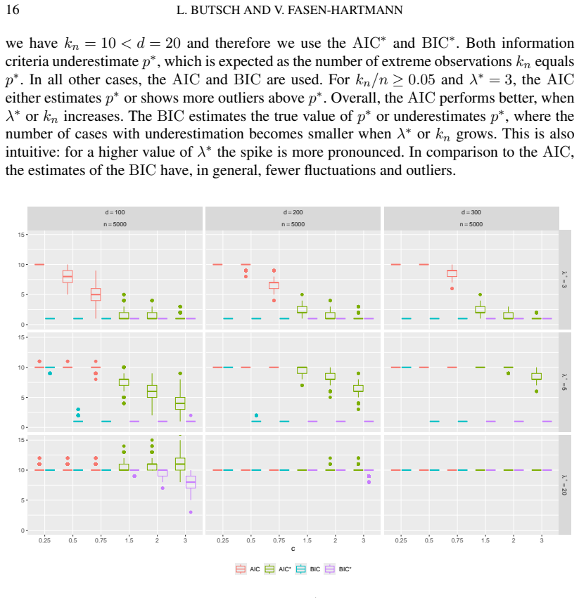
- On 500-station precipitation data, the criteria cut the dimension of extreme dependence to about 25 (AIC*) or 5–9 (BIC*), showing that the penalty choice strongly controls the resulting model size.
Reading between the lines
- A natural next step, hinted at in the paper's conclusion, is to relax the exactly-equal-trailing-eigenvalues assumption to a band of eigenvalues near the bulk edge; the same Marchenko-Pastur techniques should still give approximate consistency conditions.
- The BIC condition $\xi_{n,p^*}/\log d_n \to \infty$ suggests a practical diagnostic that the authors do not spell out: estimate the leading eigenvalue's separation from the bulk and compare it with $\log d_n$ before trusting BIC in applications.
- Because the directional model is one of several tail models, the same information-criterion analysis could be extended to other regularly varying constructions, such as hidden regular variation or kernel-based angular measures, though the paper does not do that.
Editorial analysis
A structured set of objections, weighed in public.
Referee Report
Summary. The paper proposes AIC- and BIC-type information criteria for estimating the number p* of significant principal components in the covariance matrix of the angular measure of a multivariate regularly varying random vector, under a spiked covariance assumption. Two settings are treated. In Model A, the dimension d is fixed and the number of extreme observations k_n tends to infinity with k_n/n → 0; the paper proves that the AIC is not consistent (Theorem 3.3 with a counterexample in Example 3.5) and that the BIC is weakly consistent (Theorem 3.6). In Model B, the dimension d_n increases with d_n/k_n → c ∈ (0, ∞), and the analysis is restricted to a directional model whose angular component is Γ(n)^{1/2}V / ||Γ(n)^{1/2}V||. The paper derives asymptotic results for the empirical eigenvalues (Theorems 2.7 and 2.9) and then states sufficient conditions, under 0 < c < 1 and c > 1, for AIC- and BIC-type estimators to be weakly consistent (Theorems 4.2, 4.4, 4.7, 4.8), with gap conditions (4.1) and (4.2) for the AIC and a requirement ξ_{n,p*}/log(d_n) → ∞ for the BIC. The performance of the criteria is illustrated in simulations and in an application to German precipitation data.
Significance. If the high-dimensional consistency theorems are fully established, the paper would provide the first principled, automatic method for choosing the number of principal components in multivariate extreme-value PCA, a problem that so far has been handled mainly by scree plots and risk plots. The fixed-dimensional results are clear and in line with classical information-criterion theory; the random-matrix derivations in Appendix A, in particular Theorem A.1 connecting the empirical eigenvalues of the angular measure to those of the underlying Gaussian-like matrix, are a substantive contribution. The paper also supplies code and gives a candid discussion of the restrictiveness of the spiked assumption in the precipitation application. However, the advertised high-dimensional consistency theorems are not fully proved as written, because the Appendix C proofs delegate to an external result without verifying the required uniformity over the growing candidate set. This is a load-bearing gap that must be addressed before the main claims can be accepted.
major comments (2)
- [Appendix C, proofs of Theorems 4.2, 4.4, 4.7, 4.8] The proofs of the four high-dimensional consistency theorems consist of one-paragraph statements that the proofs of Bai, Choi and Fujikoshi (2018) for bξ_{n,i} 'can be carried out step by step' for d_n λhat_{n,i}. This transfer is not automatic. The information-criterion differences involve averages of the trailing eigenvalues with lower summation index p+1 ranging over all candidate dimensions p = 1, ..., q_n, where q_n = o(d_n). Theorems 2.7(c)-(d) and 2.9(c)-(d) establish convergence of such averages only for one fixed truncation q_n = o(d_n), not uniformly over all p ≤ q_n. Controlling the argmin over the growing set {1, ..., q_n} requires simultaneous control of these statistics; pointwise convergence for each fixed p does not suffice when q_n grows. In addition, the BCF proofs are almost-sure arguments, whereas the paper only provides convergence in probability for fixed truncation points. The manuscript therefore needs either a full proof of the required sup-over-p uniformity or an explicit uniform convergence lemma showing that the replacement d_n λhat_{n,i} for bξ_{n,i} preserves the BCF arguments.
- [Section 2.1, Proposition 2.1 and Remark 2.2] Proposition 2.1, the asymptotic normality of √k_n (Σhat_n − Σ), is stated without proof; Remark 2.2 says only that the techniques of Larsson and Resnick (2012) can be generalized under the technical assumption (A4). This proposition is load-bearing: Theorem 2.3 and hence the fixed-dimensional consistency results in Section 3 (Theorems 3.3 and 3.6) rely on it. Because (A4) is a nonstandard uniform condition on truncated moments, the statement is not a routine citation, and the paper should either provide the proof or give a precise reference with the exact result covering the vectorized covariance estimator.
minor comments (5)
- [Section 5.2, noisy directional model] The model X(n) = Γ(n)^{1/2} V / ||Γ(n)^{1/2} V|| · Z + ε, with ε being entrywise absolute Gaussian noise, is used in simulations but is not shown to satisfy the directional Model B or to be multivariate regularly varying; the simulation results for this model are illustrative rather than a direct validation of the theorems.
- [Definitions 4.1 and 4.6] The definitions state p = 1, ..., d_n − 2 (or k_n − 2) but the estimator is defined as argmin over 1 ≤ p ≤ q_n; the paper should explicitly require p* ≤ q_n eventually and state how q_n is chosen in the simulations and application.
- [Section 6, Figure 8 and Section 7] The text says the scaled eigenvalue increments 'are nearly constant' after some point, but no quantitative criterion is given; the authors themselves acknowledge in Section 7 that the empirical eigenvalues do not stabilize, so the application should be framed even more explicitly as an exploratory illustration outside the spiked model.
- [Introduction, line 'Principle Component Analysis'] The phrase 'Principle Component Analysis' should be 'Principal Component Analysis'.
- [Equation (1.1) and Model B] In (1.1) the equal trailing eigenvalues are listed as λ_{p*+1} = ... = λ_{d−1}, while in the high-dimensional setting the statement in Lemma 2.5 includes λ_{dn}; the notation should be made uniform.
Circularity Check
No circular derivation: consistency proofs are built on external random-matrix theorems; the self-citation [9] is contextual and not load-bearing.
full rationale
The paper's central claims are the consistency theorems for information criteria in fixed and growing dimension. The AIC/BIC definitions are taken from Fujikoshi and Sakurai [22] and Bai, Choi and Fujikoshi [4] (external), and the asymptotic eigenvalue results in Section 2 are derived from external random matrix theory (Bai-Yin, Bai-Yao, Bai-Silverstein, Silverstein) plus the paper's own Theorem A.1, which is proven using those results. The directional model is an explicitly stated model class, not a fitted output; no parameter is calibrated to data and then presented as a prediction. In the fixed-dimensional case, Theorems 3.3 and 3.6 are proved directly from the empirical eigenvalue expansions. In the high-dimensional case, Appendix C delegates the final step to the external BCF proofs via 'step by step' replacement; however this is an appeal to an independent, prior theorem, not a self-citation, and any unverified uniformity transfer would be a proof gap rather than circularity. The only places the authors cite their own earlier work [9] are the introduction and the concluding discussion on the choice of kn; that citation is contextual and does not carry any of the consistency arguments. Simulations generate data with known p*, and the precipitation application makes no claim of recovering a fitted value. Thus there is no circular step; the derivation chain is self-contained with respect to external benchmarks.
Assumptions & free parameters
free parameters (2)
- kn (number of extreme observations) =
varies by user; 1% to 15% of n in the precipitation application
- qn (number of candidate dimensions) =
d/2 in the precipitation analysis
assumptions (6)
- domain assumption Multivariate regular variation of index α with spectral vector Θ (Model A1 and Model B1).
- domain assumption Spiked covariance structure: λ1 ≥ ... ≥ λ_{p*} > λ_{p*+1} = ... = λ_{d-1} (Eq. 1.1).
- domain assumption Directional model with i.i.d. symmetric V entries, finite fourth moment, and independent Fréchet radial part (Section 2.2).
- ad hoc to paper Technical condition (A4) on the uniform convergence of truncated moments.
- domain assumption Eigenvalue conditions: ξ_{n,p*} > 1 + √c (distant spike) or ξ_{n,p*} → ∞ with ξ_{n,1} = o(d_n^{1/2}).
- domain assumption Gaussian likelihood functional form used to define AIC and BIC.
Cite this review
Pith. "Pith review of Estimation of the number of principal components in high-dimensional multivariate extremes." pith.science (2026). https://pith.science/paper/TEAZ6T7B
@misc{pith2026250522437,
  author       = {Pith},
  title        = {Pith review of: Estimation of the number of principal components in high-dimensional multivariate extremes},
  year         = {2026},
  howpublished = {\url{https://pith.science/paper/TEAZ6T7B}},
  note         = {Machine review of arXiv:2505.22437}
}
abstract
For multivariate regularly random vectors of dimension $d$, the dependence structure of the extremes is modeled by the so-called angular measure. When the dimension $d$ is high, estimating the angular measure is challenging because of its complexity. In this paper, we use Principal Component Analysis (PCA) as a method for dimension reduction and estimate the number of significant principal components of the empirical covariance matrix of the angular measure under the assumption of a spiked covariance structure. Therefore, we develop Akaike Information Criteria (AIC) and Bayesian Information Criteria (BIC) to estimate the location of the spiked eigenvalue of the covariance matrix, reflecting the number of significant components, and explore these information criteria on consistency. On the one hand, we investigate the case where the dimension $d$ is fixed, and on the other hand, where the dimension $d$ converges to $\infty$ under different high-dimensional scenarios. When the dimension $d$ is fixed, we establish that the AIC is not consistent, whereas the BIC is weakly consistent. In the high-dimensional setting, with techniques from random matrix theory, we derive sufficient conditions for the AIC and the BIC to be consistent. Finally, the performance of the different AIC and BIC versions is compared in a simulation study and applied to high-dimensional precipitation data.
Figures


Figures from the paper (5 more)


Reference graph
Works this paper leans on
-
[1]
A KAIKE , H. (1974). A new look at the statistical model identification. IEEE Trans. Automatic Control AC-19 716–723
work page 1974
-
[2]
A NDERSON , T. W. (2003). An introduction to multivariate statistical analysis , Third ed. Wiley- Interscience
work page 2003
-
[3]
A VELLA -MEDINA , M., D AVIS, R. A. and S AMORODNITSKY , G. (2022). Kernel PCA for multivariate extremes. arXiv: 2211.13172
work page Pith review arXiv 2022
-
[4]
B AI, Z., C HOI , K. P. and F UJIKOSHI , Y. (2018). Consistency of AIC and BIC in estimating the number of significant components in high-dimensional principal component analysis. Ann. Statist. 46 1050– 1076
work page 2018
-
[5]
B AI, Z., F UJIKOSHI , Y. and H U, J. (2020). Strong consistency of the AIC, BIC, Cp and KOO methods in high-dimensional multivariate linear regression. arXiv: 1810.12609
work page Pith review arXiv 2020
-
[6]
B AI, Z. and SILVERSTEIN , J. W. (2010). Spectral analysis of large dimensional random matrices. Springer
work page 2010
-
[7]
B AI, Z. and YAO, J. (2012). On sample eigenvalues in a generalized spiked population model. J. Multivari- ate Anal. 106 167–177
work page 2012
-
[8]
B AI, Z. D. and Y IN, Y. Q. (1993). Limit of the smallest eigenvalue of a large-dimensional sample covari- ance matrix. Ann. Probab. 21 1275–1294
work page 1993
Show all 41 references
-
[9]
and F ASEN -HARTMANN , V
B UTSCH , L. and F ASEN -HARTMANN , V. (2024). Information criteria for the number of directions of ex- tremes in high-dimensional data. arxiv: 2409.10174
2024 arXiv
-
[10]
C HAUTRU , E. (2015). Dimension reduction in multivariate extreme value analysis.Electron. J. Stat. 9 383– 418. PCA FOR MULTIV ARIATE EXTREMES 37
2015
-
[11]
and S ABOURIN , A
C LÉMENÇON , S., H UET, N. and S ABOURIN , A. (2024). Regular variation in Hilbert spaces and principal component analysis for functional extremes. Stochastic Process. Appl. 174 104375
2024
-
[12]
and T HIBAUD , E
C OOLEY , D. and T HIBAUD , E. (2019). Decompositions of dependence for high-dimensional extremes. Biometrika 106 587–604
2019
-
[13]
and ROMAIN , Y
D AUXOIS , J., POUSSE , A. and ROMAIN , Y. (1982). Asymptotic theory for the principal component analysis of a vector random function: some applications to statistical inference. J. Multivariate Anal. 12 136– 154
1982
-
[14]
D AVIS, A. W. (1977). Asymptotic theory for principal component analysis: non-normal case. Austral. J. Statist. 19 206–212
1977
-
[15]
and F ERREIRA , A
DE HAAN , L. and F ERREIRA , A. (2006). Extreme Value Theory: An Introduction. Springer, New York
2006
-
[16]
D REES , H. (2025). Asymptotic Behavior of Principal Component Projections for Multivariate Extremes. arxiv: 2503.22296
2025 arXiv
-
[17]
and S ABOURIN , A
D REES , H. and S ABOURIN , A. (2021). Principal component analysis for multivariate extremes. Electron. J. Stat. 15 908–943
2021
-
[18]
Daily station observations precipitation height in mm for Germany, version v21.3, last accessed: May 03, 2023
DWD-C LIMATE -DATA-CENTER -(CDC) (1951 - 2022). Daily station observations precipitation height in mm for Germany, version v21.3, last accessed: May 03, 2023
1951
-
[19]
and P E ˘CARI ´C, J
E LEZOVI ´C, N., G IORDANO , C. and P E ˘CARI ´C, J. (2000). The best bounds in Gautschi’s inequality. Math. Inequal. Appl. 3 239–252
2000
-
[20]
and I VANOVS , J
E NGELKE , S. and I VANOVS , J. (2021). Sparse structures for multivariate extremes. Annu. Rev. Stat. Appl. 8 241–270
2021
-
[21]
F ALK , M. (2019). Multivariate extreme value theory and D-norms. Springer Series in Operations Research and Financial Engineering. Springer, Cham
2019
-
[22]
and SAKURAI , T
F UJIKOSHI , Y. and SAKURAI , T. (2016). Some properties of estimation criteria for dimensionality in Prin- cipal Component Analysis. AJMMS 35 133-142
2016
-
[23]
V., M CKEAN , J
H OGG , R. V., M CKEAN , J. W. and C RAIG , A. T. (2005). Introduction to mathematical statistics , 6. ed. Pearson Prentice Hall
2005
-
[24]
H ORN , R. A. and J OHNSON , C. R. (2013). Matrix analysis, Second ed. Cambridge University Press
2013
-
[25]
and L I, Z
J IANG , Q., Q IU, J. and L I, Z. (2023). On eigenvalues of sample covariance matrices based on high dimen- sional compositional data. arXiv : 2312.14420
2023 arXiv
-
[26]
J OHNSTONE , I. M. (2001). On the distribution of the largest eigenvalue in principal components analysis. Ann. Statist. 29 295–327
2001
-
[27]
J OHNSTONE , I. M. and Y ANG , J. (2018). Notes on asymptotics of sample eigenstructure for spiked covari- ance models with non-Gaussian data. arXiv : 1810.10427
2018 arXiv
-
[28]
and R ESNICK , S
L ARSSON , M. and R ESNICK , S. I. (2012). Extremal dependence measure and extremogram: the regularly varying case. Extremes 15 231–256
2012
-
[29]
M AR ˇCENKO , V. A. and PASTUR , L. A. (1967). Distribution of eigenvalues for some sets of random matri- ces. Mat. Sb. 1 457
1967
-
[30]
and W INTENBERGER , O
M EYER , N. and W INTENBERGER , O. (2023). Multivariate sparse clustering for extremes. J. Amer. Statist. Assoc. 0 1-12
2023
-
[31]
M UIRHEAD , R. J. (1982). Aspects of multivariate statistical theory. John Wiley & Sons, Inc
1982
-
[32]
P AUL, D. (2007). Asymptotics of sample eigenstructure for a large dimensional spiked covariance model. Statist. Sinica 17 1617–1642
2007
-
[33]
R ESNICK , S. I. (1987). Extreme Values, Regular Variation, and Point Processes. Springer
1987
-
[34]
R ESNICK , S. I. (2007). Heavy-Tail Phenomena: Probabilistic and Statistical Modeling. Springer
2007
-
[35]
and C OOLEY , D
R OHRBECK , C. and C OOLEY , D. (2023). Simulating flood event sets using extremal principal components. Ann. Appl. Stat. 17 1333–1352
2023
-
[36]
S CHWARZ , G. (1978). Estimating the dimension of a model. Ann. Statist. 6 461–464
1978
-
[37]
S ILVERSTEIN , J. W. (1995). Strong convergence of the empirical distribution of eigenvalues of large- dimensional random matrices. J. Multivariate Anal. 55 331–339
1995
-
[38]
S ILVERSTEIN , J. W. and C HOI , S.-I. (1995). Analysis of the limiting spectral distribution of large- dimensional random matrices. J. Multivariate Anal. 54 295–309
1995
-
[39]
U CHIDA , Y. (2008). A simple proof of the geometric-arithmetic mean inequality. J. Inequal. Pure Appl. Math. 9
2008
-
[40]
W AN, P. (2024). Characterizing extremal dependence on a hyperplane. arxiv:2411.00573
2024
-
[41]
Q., B AI, Z
Y IN, Y. Q., B AI, Z. D. and K RISHNAIAH , P. R. (1988). On the limit of the largest eigenvalue of the large-dimensional sample covariance matrix. Probab. Theory Related Fields78 509–521
1988
Reviewed August 7, 2026 · model on record in the stance chip above.
Discussion (0). Sign in to comment.