REVIEW 4 major objections 5 minor 66 references
Global resistive MHD accretion flows around spinning AGNs: impact of resistivity on MAD state
T0 review · 4 major / 5 minor · reviewed 2026-08-07 · deepseek-v4-flash
Pith's one-line read Resistive accretion flows around spinning black holes all settle into the magnetically arrested state, and a domain-averaged plasma beta at or below one marks the transition.
desk verdict A competent resistive-MHD parameter study whose robust MAD core is undercut by an undefined, floor-sensitive beta_ave diagnostic presented as the main new result. read the letter →
The pith
A machine-rendered reading of the paper's core claim, the machinery that carries it, and where it could break.
The reading
What carries the argument
The load-bearing object is the pair of MAD indicators: the normalized magnetic flux threading the inner boundary, $\dot{\phi}_{\rm acc}$, previously used to define the MAD threshold, and the newly proposed volume-averaged plasma $\beta$ $\beta_{\rm ave}$ computed over the whole computational domain. The paper's argument runs on the correspondence between these two: whenever $\dot{\phi}_{\rm acc}$ rises above the canonical value of about 50, $\beta_{\rm ave}$ falls to or below unity, so the averaged pressure ratio serves as a proxy for the horizon-flux criterion. The simulations are driven by a resistive MHD code with an effective Kerr potential, uniform resistivity, and a fixed torus set to MAD-like dimensions; the MRI quality factor, Maxwell and Reynolds stresses, and current density maps carry the secondary claims about turbulence and reconnection.
What would settle it
Rerun one low- and one high-resistivity model with the density and pressure floors lowered by at least two orders of magnitude and with $\beta_{\rm ave}$ recomputed both over the full domain and over the disk body only; if the horizon flux still exceeds the MAD threshold while the disk-restricted $\beta_{\rm ave}$ stays above one, the proposed criterion is an artifact of the floor-dominated averaging volume.
Extended reading notes
Core claim
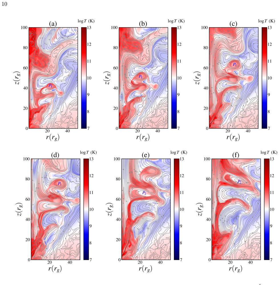
The central claim is that resistivity does not destroy the magnetically arrested state: all resistive models considered, with uniform resistivity from about 0 to 0.1, reach the MAD state as measured by the normalized horizon magnetic flux $\dot{\phi}_{\rm acc}$ crossing the canonical threshold of about 50 in Gaussian units. The paper's new proposal is that this state can be identified from the spatial average of the plasma $\beta$, $\beta_{\rm ave}$, computed over the entire computational domain; the flow enters MAD when $\beta_{\rm ave} \lesssim 1$, meaning magnetic pressure is comparable to or larger than gas pressure on average. The same simulations show that mass accretion rates are nearly equal in 2D and 3D until $t \approx 1000\,t_g$ and then diverge as non-axisymmetric MRI turbulence dominates in 3D, that high resistivity ($\eta = 0.1, 0.01$) damps MRI turbulence, that low-resistivity runs show plasmoids and current sheets in the jet region, that variability of accretion rate and magnetic flux shows no clear trend with resistivity, and that jet power is roughly two orders of magnitude lower at $\eta = 0.1$ than at $\eta \leq 10^{-3}$.
Load-bearing premise
The criterion rests on the assumption that averaging the plasma beta over the whole simulation box, including the very low-density, low-pressure atmosphere used to fill empty space, measures the disk's true magnetization rather than being dominated by the artificial floor values.
Editorial extensions
If this is right
- A volume-averaged plasma beta at or below unity can be used as a practical MAD indicator in global simulations, without computing horizon-threading flux.
- Resistivity by itself does not select the magnetic state; even strongly diffusive flows accumulate enough flux to become MAD, so comparisons of MAD versus non-MAD flows should not be attributed to resistivity.
- In any model with high resistivity, jet power is expected to be about two orders of magnitude weaker, because less magnetic flux accumulates at the horizon.
- Simulations aiming at late-time accretion behavior must be three-dimensional after $t \approx 1000\,t_g$, when non-axisymmetric effects change the accretion rate and flux.
- Low-resistivity flows are the places to look for reconnection-driven plasmoid formation in jets, though the resolution here is insufficient to confirm the plasmoid dynamics.
Reading between the lines
- The $\beta_{\rm ave} \lesssim 1$ threshold would be on firmer ground if recomputed as a mass-weighted or disk-restricted average; the current volume average includes floor-dominated atmosphere, and the authors do not report such a test.
- If the threshold survives, it suggests a purely local pressure-balance criterion for MAD that could be applied to observed accretion flows via inferred magnetic and gas pressures, not just to simulations.
- The absence of a variability-resistivity trend hints that observed timing variability in sources like Sgr A* is set by something other than the effective magnetic diffusivity, for instance the intermittent flux-eruption cycle common to MAD states.
- The plasmoid formation at low resistivity in jets suggests that reconnection-powered flares should be more prominent in low-diffusivity sources; correlating flaring activity with jet power in AGN samples would test this.
Editorial analysis
A structured set of objections, weighed in public.
Referee Report
Summary. This paper presents global resistive MHD simulations of magnetized accretion flows around a spinning black hole, using the PLUTO code with an effective Kerr potential. The authors run two-dimensional axisymmetric and three-dimensional models with uniform resistivities from η=0.1 down to the ideal-MHD limit, and compare mass accretion rates, normalized horizon magnetic flux, MRI quality factors, stresses, variability, and jet power. They report that all models reach the magnetically arrested disk (MAD) state according to the standard horizon-flux criterion φ_acc ≳ 50, and they propose that a spatial average plasma beta β_ave ≲ 1 over the computational domain is an alternative indicator of the MAD state. Additional results include reduced MRI turbulence and jet power at high resistivity, plasmoid formation at low resistivity, and no clear resistivity-variability correlation.
Significance. If substantiated, the β_ave ≲ 1 criterion would be an inexpensive diagnostic for classifying MAD versus non-MAD states in global simulations, and the resistivity-dependent trends (turbulence suppression, jet-power reduction, plasmoid formation) are timely for interpreting EHT and GRAVITY observations. The paper also provides a useful 2D versus 3D comparison at higher effective resolution than typical GRMHD runs. The main weakness is that the proposed β_ave diagnostic is not defined operationally and lacks sensitivity tests; as presented, the central claim is not sufficiently supported.
major comments (4)
- [Section 3, Fig. 2c] The manuscript never defines how β_ave is computed. The text says "spatial average plasma-beta parameter across the entire computational domain," but no equation or weighting is given (e.g., volume-weighted arithmetic mean of β, ratio of volume-averaged pressures, or mass-weighted average). Because the domain is largely filled by the low-density atmosphere at the numerical floors ρ_floor=10^-6 ρ0 and P_floor=10^-8 P0 (Section 2.6), a whole-domain average can be sensitive to the floor values; the paper presents no sensitivity test to floors, domain size, or weighting scheme. The conclusion that β_ave ≲ 1 signals the MAD state is therefore not established and could be an artifact of the atmosphere treatment.
- [Section 3, Fig. 2c vs 2b] The threshold β_ave=1 is read off from the same set of simulations used to classify the MAD state via φ_acc≥50. This is a post-hoc correlation rather than an independent test. To support the claim, the authors should validate the threshold on a held-out set of simulations or on subregions of the same runs (e.g., excluding the atmosphere), and show that the crossing time of β_ave=1 tracks φ_acc=50 under different floor settings.
- [Section 3, Figs. 3 and 4] The MRI quality factors and the Maxwell/Reynolds stress profiles are computed at a single time t=8500 tg and, for the 3D models, at a single azimuthal slice φ=0. In a turbulent flow these diagnostics fluctuate strongly in time and azimuth; the reported factors-of-1000 differences between 2D and 3D models near the black hole are not robust without time/azimuth averaging. This does not affect the time-series conclusions from Fig. 2, but it weakens the quantitative turbulence comparison.
- [Section 2.7 and Fig. 2b] The normalized flux φ_acc is defined in Gaussian units but the y-axis of Fig. 2b is labeled "code unit." The conversion between the code's magnetic field units (where P_mag=B²/2) and the Gaussian-unit threshold φ_acc=50 is not stated. Without this conversion the reader cannot verify whether the plotted curves actually cross the MAD threshold; please clarify the units and conversion factors.
minor comments (5)
- [Section 2.3] The atmosphere profile ρ_atm = ρ_floor r^{-3/2}, P_atm = P_floor r^{-5/2} appears to use the same floor constants as the numerical floors in Section 2.6; for r>1 this puts the initial atmosphere below the floor, so the floor will override it. Please clarify how the atmosphere and the floor are meant to interact.
- [Section 2.5] The computational domain extent (r_min, r_max, z_max) is not stated; only the inner boundary and resolution are given. The domain size is needed to interpret the phrase "entire computational domain" and the volume averages.
- [Section 4] The discussion of limitations focuses on resolution for reconnection and plasmoids, but does not mention the sensitivity of β_ave to numerical floors; this omission should be addressed in the revision.
- [References] The reference "SÄ dowski" should be "Sądowski".
- [Figure 5 and Figure 8] The color maps and line styles for resistivity values η=10^-4 and η=10^-5 are hard to distinguish; consider labeling each panel with the η value more prominently and using a perceptually uniform colormap.
Circularity Check
No significant circularity: the MAD classification rests on an external φ_acc threshold, and the β_ave≤1 criterion is an in-sample empirical indicator, not a definitional or fitted substitute.
full rationale
No circular step is exhibited in the paper's derivation chain. The MAD classification is anchored to an externally established threshold, φ_acc ≳ 50 in Gaussian units (Section 2.7), with φ_acc computed from the horizon radial magnetic field and mass accretion rate via Eqs. (11)–(14). The proposed β_ave diagnostic is a distinct quantity, and the statement that 'βave ≲ 1 when the flow transitions into the MAD state' (Section 3) is presented as an empirical correlation used as an indicator, not as the definition of MAD; the paper does not use β_ave to define the MAD state. Self-citations to R. Aktar et al. 2024a,b are methodological (effective Kerr potential implementation, torus initialization, MRI quality factor) and are not load-bearing for the central MAD conclusion, which is validated by comparison with the literature threshold for φ_acc. The β_ave criterion is not formally defined by an explicit averaging equation, and it may be sensitive to the atmosphere floor values and domain size; however, these are correctness and robustness concerns, not circular reductions, and the acknowledged resolution limitation in Section 4 does not itself indicate a circular step. Overall, no claim in the paper reduces to its own input by construction, so the appropriate circularity score is 0.
Assumptions & free parameters
free parameters (4)
- MAD threshold on average plasma beta =
<= 1 (dimensionless)
- BZ jet power coefficient kappa =
0.1
- Numerical floor density and pressure =
rho_floor = 1e-6 rho_0, P_floor = 1e-8 P_0
- Initial torus and magnetic configuration =
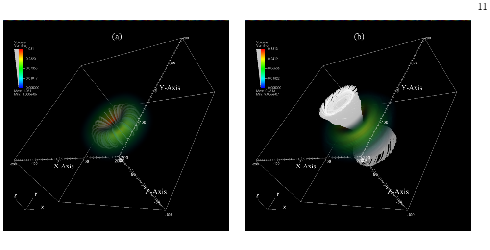
r_min = 20 rg, r_max = 40 rg, beta_0 = 10, a_k = 0.95, lambda = 6.2
assumptions (4)
- domain assumption Resistive MHD equations with a diagonal, globally uniform resistivity tensor describe accretion-flow reconnection adequately.
- domain assumption The effective Kerr potential of Eq. (6) captures the essential spacetime features for MAD flux accumulation and jets.
- domain assumption The normalized magnetic flux threshold phi_dot >= 50 defines the MAD state in this pseudo-Newtonian model.
- domain assumption The Blandford-Znajek jet power expression P_jet = kappa phi^2 Omega_H^2 with kappa=0.1 applies to these simulations.
Cite this review
Pith. "Pith review of Global resistive MHD accretion flows around spinning AGNs: impact of resistivity on MAD state." pith.science (2026). https://pith.science/paper/CWIRAK3U
@misc{pith2026250523051,
  author       = {Pith},
  title        = {Pith review of: Global resistive MHD accretion flows around spinning AGNs: impact of resistivity on MAD state},
  year         = {2026},
  howpublished = {\url{https://pith.science/paper/CWIRAK3U}},
  note         = {Machine review of arXiv:2505.23051}
}
abstract
In this study, we investigate the effect of resistivity on the dynamics of global magnetohydrodynamic accretion flows (Res-MHD) around a spinning supermassive black hole. We perform a comparative study of 2D and 3D resistive models around black holes. We examine accretion flow dynamics considering globally uniform resistivity values, ranging from $\sim 0$ to 0.1. During the simulation time of $t \lesssim 1000~t_g$, we find that the mass accretion rate is comparable for both the 2D and 3D models. However, as the flow becomes increasingly turbulent, non-axisymmetric effects begin to dominate, resulting in significant differences in the mass accretion rates between the 3D and 2D. All the resistive models in a highly magnetized flow belong to the Magnetically Arrested Disk (MAD) state. We propose an efficient and physically motivated approach to examine the magnetic state by estimating the spatial average plasma beta parameter across the computational domain. We find that when the average plasma beta is close to or below unity $( \beta_{\text{ave}} \lesssim 1 )$, the accretion flow enters the MAD state. Additionally, we find that high-resistivity flow reduces magnetorotational instability (MRI) turbulence in the accretion flow, while the turbulence structures remain qualitatively similar in low-resistivity flows. Moreover, we observe indications of plasmoid formations in low-resistivity flow compared to high-resistivity flow. Furthermore, we do not find a clear relationship between the variability of the accretion rate, magnetic flux, and resistivity. Lastly, our findings suggest that low-resistivity models produce higher power jets than those with higher resistivity.
Figures


Figures from the paper (6 more)




Reference graph
Works this paper leans on
-
[1]
1978, A&A, 63, 221
Abramowicz, M., Jaroszynski, M., & Sikora, M. 1978, A&A, 63, 221
1978
-
[2]
2024a, MNRAS, 527, 1745, doi: 10.1093/mnras/stad3287
Aktar, R., Pan, K.-C., & Okuda, T. 2024a, MNRAS, 527, 1745, doi: 10.1093/mnras/stad3287
-
[3]
2024b, ApJ, 972, 18, doi: 10.3847/1538-4357/ad5a8a Alfvén, H
Aktar, R., Pan, K.-C., & Okuda, T. 2024b, ApJ, 972, 18, doi: 10.3847/1538-4357/ad5a8a Alfvén, H. 1942, Nature, 150, 405, doi: 10.1038/150405d0
-
[4]
Baganoff, F. K., Bautz, M. W., Brandt, W. N., et al. 2001, Nature, 413, 45, doi: 10.1038/35092510
doi:10.1038/35092510 2001
-
[5]
Balbus, S. A., & Hawley, J. F. 1991, ApJ, 376, 214, doi: 10.1086/170270
doi:10.1086/170270 1991
-
[6]
2016, ApJ, 826, 77, doi: 10.3847/0004-637X/826/1/77
Ball, D., Özel, F., Psaltis, D., & Chan, C.-k. 2016, ApJ, 826, 77, doi: 10.3847/0004-637X/826/1/77
-
[7]
2018, ApJ, 853, 184, doi: 10.3847/1538-4357/aaa42f
Ball, D., Özel, F., Psaltis, D., Chan, C.-K., & Sironi, L. 2018, ApJ, 853, 184, doi: 10.3847/1538-4357/aaa42f
-
[8]
Blandford, R. D., & Znajek, R. L. 1977, MNRAS, 179, 433, doi: 10.1093/mnras/179.3.433
Show all 66 references
-
[9]
2019, ApJ, 871, 161, doi: 10.3847/1538-4357/aaf71f
Boyce, H., Haggard, D., Witzel, G., et al. 2019, ApJ, 871, 161, doi: 10.3847/1538-4357/aaf71f
2019 doi
-
[10]
2022, ApJ, 941, 30, doi: 10.3847/1538-4357/ac9d97
Chatterjee, K., & Narayan, R. 2022, ApJ, 941, 30, doi: 10.3847/1538-4357/ac9d97
2022 doi
-
[11]
Cowling, T. G. 1933, MNRAS, 94, 39, doi: 10.1093/mnras/94.1.39
1933 doi
-
[12]
2023, Nature, 621, 711, doi: 10.1038/s41586-023-06479-6
Cui, Y., Hada, K., Kawashima, T., et al. 2023, Nature, 621, 711, doi: 10.1038/s41586-023-06479-6
2023 doi
-
[13]
2023, MNRAS, 518, 3441, doi: 10.1093/mnras/stac3330
Curd, B., & Narayan, R. 2023, MNRAS, 518, 3441, doi: 10.1093/mnras/stac3330
2023 doi
-
[14]
M., Kennea, J., et al
Degenaar, N., Miller, J. M., Kennea, J., et al. 2013, ApJ, 769, 155, doi: 10.1088/0004-637X/769/2/155
2013 doi
-
[15]
Dhang, P., Bai, X.-N., & White, C. J. 2023, ApJ, 944, 182, doi: 10.3847/1538-4357/acb534
2023 doi
-
[16]
N., & Gammie, C
Dhruv, V., Prather, B., Wong, G. N., & Gammie, C. F. 2025, ApJS, 277, 16, doi: 10.3847/1538-4365/adaea6
2025 doi
-
[17]
K., Das, S., Maity, D., & Chakrabarti, S
Dihingia, I. K., Das, S., Maity, D., & Chakrabarti, S. 2018, PhRvD, 98, 083004, doi: 10.1103/PhysRevD.98.083004
2018 doi
-
[18]
K., Vaidya, B., & Fendt, C
Dihingia, I. K., Vaidya, B., & Fendt, C. 2021, MNRAS, 505, 3596, doi: 10.1093/mnras/stab1512
2021 doi
-
[19]
K., Vaidya, B., & Fendt, C
Dihingia, I. K., Vaidya, B., & Fendt, C. 2022, MNRAS, 517, 5032, doi: 10.1093/mnras/stac3021 Event Horizon Telescope Collaboration, Akiyama, K.,
2022 doi
-
[20]
2019, ApJL, 875, L1, doi: 10.3847/2041-8213/ab0ec7 Event Horizon Telescope Collaboration, Akiyama, K.,
Alberdi, A., et al. 2019, ApJL, 875, L1, doi: 10.3847/2041-8213/ab0ec7 Event Horizon Telescope Collaboration, Akiyama, K.,
2019 doi
-
[21]
C., et al
Algaba, J. C., et al. 2021, ApJL, 910, L13, doi: 10.3847/2041-8213/abe4de Event Horizon Telescope Collaboration, Akiyama, K.,
2021 doi
-
[22]
2022, ApJL, 930, L12, doi: 10.3847/2041-8213/ac6674 Event Horizon Telescope Collaboration, Akiyama, K.,
Alberdi, A., et al. 2022, ApJL, 930, L12, doi: 10.3847/2041-8213/ac6674 Event Horizon Telescope Collaboration, Akiyama, K.,
2022 doi
-
[23]
2024, ApJL, 964, L26, doi: 10.3847/2041-8213/ad2df1
Alberdi, A., et al. 2024, ApJL, 964, L26, doi: 10.3847/2041-8213/ad2df1
2024 doi
-
[24]
G., Hora, J
Fazio, G. G., Hora, J. L., Witzel, G., et al. 2018, ApJ, 864, 58, doi: 10.3847/1538-4357/aad4a2
2018 doi
-
[25]
M., Cruz-Osorio, A., Mizuno, Y., et al
Fromm, C. M., Cruz-Osorio, A., Mizuno, Y., et al. 2022, A&A, 660, A107, doi: 10.1051/0004-6361/202142295
2022 doi
-
[26]
F., McKinney, J
Gammie, C. F., McKinney, J. C., & Tóth, G. 2003, ApJ, 589, 444, doi: 10.1086/374594
2003 doi
-
[27]
2003, Nature, 425, 934, doi: 10.1038/nature02065 GRAVITY Collaboration, Abuter, R., Amorim, A., et al
Genzel, R., Schödel, R., Ott, T., et al. 2003, Nature, 425, 934, doi: 10.1038/nature02065 GRAVITY Collaboration, Abuter, R., Amorim, A., et al. 2018, A&A, 618, L10, doi: 10.1051/0004-6361/201834294 17 GRAVITY Collaboration, Bauböck, M., Dexter, J., et al. 2020, A&A, 635, A143,...
2003 doi
-
[28]
Hawley, J. F. 2000, ApJ, 528, 462, doi: 10.1086/308180
2000 doi
-
[29]
F., Guan, X., & Krolik, J
Hawley, J. F., Guan, X., & Krolik, J. H. 2011, ApJ, 738, 84, doi: 10.1088/0004-637X/738/1/84
2011 doi
- [30]
- [31]
-
[32]
F., Richers, S
Hawley, J. F., Richers, S. A., Guan, X., & Krolik, J. H. 2013, ApJ, 772, 102, doi: 10.1088/0004-637X/772/2/102
2013 doi
-
[33]
Igumenshchev, I. V. 2008, ApJ, 677, 317, doi: 10.1086/529025
2008 doi
-
[34]
2022, A&A, 668, A66, doi: 10.1051/0004-6361/202244196
Janiuk, A., & James, B. 2022, A&A, 668, A66, doi: 10.1051/0004-6361/202244196
2022 doi
-
[35]
M., & Nathanail, A
Jiang, H.-X., Mizuno, Y., Fromm, C. M., & Nathanail, A. 2023, MNRAS, 522, 2307, doi: 10.1093/mnras/stad1106
2023 doi
-
[36]
A., & Livio, M
Junor, W., Biretta, J. A., & Livio, M. 1999, Nature, 401, 891, doi: 10.1038/44780
1999 doi
-
[37]
2005, ApJ, 621, 921, doi: 10.1086/427720
Kuwabara, T., Shibata, K., Kudoh, T., & Matsumoto, R. 2005, ApJ, 621, 921, doi: 10.1086/427720
2005 doi
-
[38]
2018, MNRAS, 474, L81, doi: 10.1093/mnrasl/slx174
Liska, M., Hesp, C., Tchekhovskoy, A., et al. 2018, MNRAS, 474, L81, doi: 10.1093/mnrasl/slx174
2018 doi
-
[39]
1996, ApJ, 461, 115, doi: 10.1086/177041
Matsumoto, R., Uchida, Y., Hirose, S., et al. 1996, ApJ, 461, 115, doi: 10.1086/177041
1996 doi
-
[41]
2008, ApJL, 688, L17, doi: 10.1086/593147
Meyer, L., Do, T., Ghez, A., et al. 2008, ApJL, 688, L17, doi: 10.1086/593147
2008 doi
-
[42]
2007, ApJS, 170, 228, doi: 10.1086/513316
Mignone, A., Bodo, G., Massaglia, S., et al. 2007, ApJS, 170, 228, doi: 10.1086/513316
2007 doi
-
[43]
M., Younsi, Z., et al
Mizuno, Y., Fromm, C. M., Younsi, Z., et al. 2021, MNRAS, 506, 741, doi: 10.1093/mnras/stab1753
2021 doi
-
[44]
2022, MNRAS, 511, 3795, doi: 10.1093/mnras/stac285
Curd, B. 2022, MNRAS, 511, 3795, doi: 10.1093/mnras/stac285
2022 doi
-
[45]
V., & Abramowicz, M
Narayan, R., Igumenshchev, I. V., & Abramowicz, M. A. 2003, PASJ, 55, L69, doi: 10.1093/pasj/55.6.L69
2003 doi
-
[46]
F., & Kulkarni, A
Narayan, R., SÄ dowski, A., Penna, R. F., & Kulkarni, A. K. 2012, MNRAS, 426, 3241, doi: 10.1111/j.1365-2966.2012.22002.x
2012
-
[47]
M., Porth, O., et al
Nathanail, A., Fromm, C. M., Porth, O., et al. 2020, MNRAS, 495, 1549, doi: 10.1093/mnras/staa1165
2020 doi
- [48]
-
[49]
A., Gammie, C., et al
Neilsen, J., Nowak, M. A., Gammie, C., et al. 2013, ApJ, 774, 42, doi: 10.1088/0004-637X/774/1/42
2013 doi
-
[50]
A., et al
Neilsen, J., Markoff, S., Nowak, M. A., et al. 2015, ApJ, 799, 199, doi: 10.1088/0004-637X/799/2/199
2015 doi
-
[51]
B., & Aktar, R
Okuda, T., Singh, C. B., & Aktar, R. 2022, MNRAS, 514, 5074, doi: 10.1093/mnras/stac1630
2022 doi
-
[52]
B., & Aktar, R
Okuda, T., Singh, C. B., & Aktar, R. 2023, MNRAS, 522, 1814, doi: 10.1093/mnras/stad1096
2023 doi
-
[53]
B., Das, S., et al
Okuda, T., Singh, C. B., Das, S., et al. 2019, PASJ, 71, 49, doi: 10.1093/pasj/psz021
2019 doi
-
[54]
R., et al
Ponti, G., De Marco, B., Morris, M. R., et al. 2015, MNRAS, 454, 1525, doi: 10.1093/mnras/stv1537
2015 doi
-
[55]
2017, Computational Astrophysics and Cosmology, 4, 1, doi: 10.1186/s40668-017-0020-2
Porth, O., Olivares, H., Mizuno, Y., et al. 2017, Computational Astrophysics and Cosmology, 4, 1, doi: 10.1186/s40668-017-0020-2
2017 doi
-
[56]
Proga, D., & Begelman, M. C. 2003, ApJ, 582, 69, doi: 10.1086/344537
2003 doi
-
[57]
Ripperda, B., Bacchini, F., & Philippov, A. A. 2020, ApJ, 900, 100, doi: 10.3847/1538-4357/ababab
2020 doi
-
[58]
2022, ApJL, 924, L32, doi: 10.3847/2041-8213/ac46a1
Ripperda, B., Liska, M., Chatterjee, K., et al. 2022, ApJL, 924, L32, doi: 10.3847/2041-8213/ac46a1
2022 doi
-
[59]
2019, ApJS, 244, 10, doi: 10.3847/1538-4365/ab3922
Ripperda, B., Bacchini, F., Porth, O., et al. 2019, ApJS, 244, 10, doi: 10.3847/1538-4365/ab3922
2019 doi
-
[60]
M., & Pringle, J
Stone, J. M., & Pringle, J. E. 2001, MNRAS, 322, 461, doi: 10.1046/j.1365-8711.2001.04138.x
2001
-
[61]
Tchekhovskoy, A., Narayan, R., & McKinney, J. C. 2010, ApJ, 711, 50, doi: 10.1088/0004-637X/711/1/50
2010 doi
-
[62]
Tchekhovskoy, A., Narayan, R., & McKinney, J. C. 2011, MNRAS, 418, L79, doi: 10.1111/j.1745-3933.2011.01147.x
2011
-
[63]
Vourellis, C., Fendt, C., Qian, Q., & Noble, S. C. 2019, ApJ, 882, 2, doi: 10.3847/1538-4357/ab32e2
2019 doi
-
[64]
J., Stone, J
White, C. J., Stone, J. M., & Gammie, C. F. 2016, ApJS, 225, 22, doi: 10.3847/0067-0049/225/2/22
2016 doi
-
[65]
J., Stone, J
White, C. J., Stone, J. M., & Quataert, E. 2019, ApJ, 874, 168, doi: 10.3847/1538-4357/ab0c0c
2019 doi
-
[66]
N., Du, Y., Prather, B
Wong, G. N., Du, Y., Prather, B. S., & Gammie, C. F. 2021, ApJ, 914, 55, doi: 10.3847/1538-4357/abf8b8
2021 doi
-
[67]
Q., Bégué, D., Pe’er, A., & Zhang, B
Zhang, G. Q., Bégué, D., Pe’er, A., & Zhang, B. B. 2024, ApJ, 962, 135, doi: 10.3847/1538-4357/ad167b
2024 doi
Reviewed August 7, 2026 · model on record in the stance chip above.
Discussion (0). Sign in to comment.