REVIEW 3 major objections 5 minor 38 references
State Space Model Programming in Turing.jl
T0 review · 3 major / 5 minor · reviewed 2026-08-07 · deepseek-v4-flash
Pith's one-line read A single state-space model definition can drive Kalman, particle, Rao-Blackwellised, and GPU-accelerated inference, with the paper reporting a 79.4x GPU speed-up on a particle benchmark.
desk verdict A serious software paper with a genuinely useful interface design; the GPU scalability claim is real but only demonstrated on one linear-Gaussian benchmark. read the letter →
The pith
A machine-rendered reading of the paper's core claim, the machinery that carries it, and where it could break.
The reading
What carries the argument
The load-bearing mechanism is the interface, not any single numerical identity. SSMProblems.jl defines an SSM as a LatentDynamics object plus an ObservationProcess object, each supplying distribution (or simulate/logdensity) methods, with LinearGaussianLatentDynamics additionally exposing calc_A, calc_b, and calc_Q for closed-form access. GeneralisedFilters.jl defines inference as predict and update methods that return a distribution-like ParticleContainer together with the incremental log-likelihood. These pieces compose: hierarchical SSMs, built by wrapping an inner model with outer dynamics and passing prev_outer/new_outer keyword arguments, make arbitrary Rao-Blackwellisation expressible, and a generic step and filter function makes PMMH a one-line change of inner algorithm.
What would settle it
Re-run the same package's GPU and CPU RBPF benchmark on a nonlinear state space model, for example the Lorenz observer from the paper's appendix, with $10^{5}$ particles and with resampling and data-dependent transitions inside the timed step; if GPU wall time per step rises with particle count rather than staying flat near the CPU time, the claimed generic GPU advantage is falsified for that workload.
Extended reading notes
Core claim
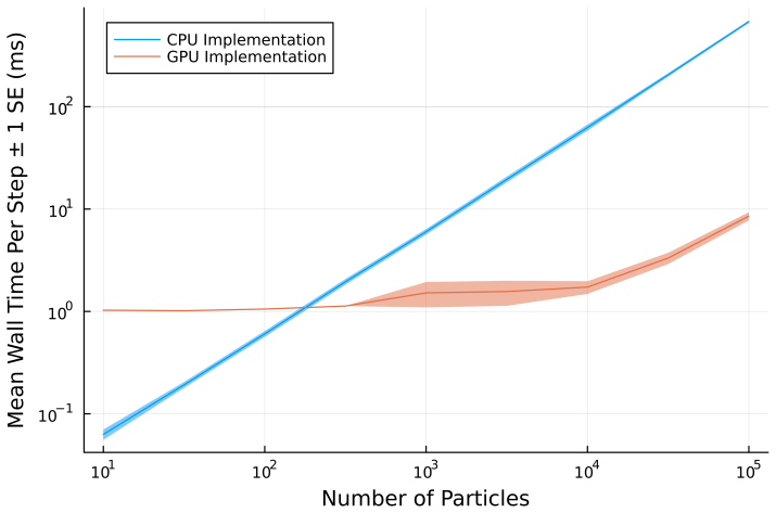
The central discovery is a consistency argument: filtering algorithms can be written entirely in terms of two modular operations, predict and update, that both accept and return a distribution-like object such as a Gaussian or a weighted particle set. Given that discipline, a model specified once in SSMProblems.jl can be handed to any algorithm, exact or approximate; a Rao-Blackwellised particle filter is just an RBPF object whose inner algorithm can be any other filter, and particle MCMC is the generic filter function embedded in a Metropolis-Hastings step. The paper reports that this design is not only convenient but fast: on the GPU benchmark, wall time per predict-update step stays nearly flat as particle count rises, giving a 79.4x speed-up at $10^{5}$ particles over the serial CPU implementation.
Load-bearing premise
The load-bearing premise is that the uniform, branch-free linear algebra of the benchmarked linear-Gaussian RBPF represents what typical SSM workloads look like; if realistic nonlinear models with per-particle divergence do not have that structure, the reported 40-79x GPU speed-ups will not transfer.
Editorial extensions
If this is right
- A single model definition is enough to compare a Kalman filter, a bootstrap particle filter, and a Rao-Blackwellised particle filter, so benchmarking candidate inference methods no longer requires reimplementation.
- Particle MCMC can be run with any inner filter by changing one algorithm type, and with a Kalman filter the same code performs exact rather than pseudo-marginal Metropolis-Hastings.
- Rao-Blackwellisation is no longer locked to linear-Gaussian substructures; any inner filter, such as the forward algorithm or an extended Kalman filter, can be swapped in.
- GPU-accelerated filtering is available for batched Kalman, square-root Kalman, forward algorithm, and particle filters, with the RBPF inheriting the speed-up by composition.
- The reported 79.4x speed-up at 10^5 particles is accompanied by roughly 40x performance gains already at 10^4 particles on the paper's benchmark.
Reading between the lines
- Because the benchmark model is linear-Gaussian with dense matrices, all 10^5 particles execute the same branch-free linear algebra; realistic nonlinear models with data-dependent dynamics and per-particle resampling are likely to show smaller GPU gains, and measuring that gap would be a natural stress test.
- The same predict/update composition could extend naturally to smoothing algorithms and to SMC^2, since both are built from filtering likelihoods and particle genealogies.
- The sparse particle path storage used in the trend-inflation case study supports approximate smoothing; a systematic comparison against MCMC-based smoothed estimates would test how faithful that approximation is.
- If the interface were adopted as a common model description, other state-space software could target it, making 'define once, infer many ways' a cross-library standard rather than a Julia-internal one.
Editorial analysis
A structured set of objections, weighed in public.
Referee Report
Summary. The paper introduces two Julia packages, SSMProblems.jl and GeneralisedFilters.jl, which provide a unified and composable interface for defining state space models and performing inference on them. The interface is designed so that a single model definition can be used with Kalman filtering, particle filtering, Rao-Blackwellised particle filters, particle MCMC, and GPU-accelerated inference. The central claim is that this framework is consistent, composable, general, and scalable. Evidence includes complete code listings, a GPU benchmark reporting a 79.4x speedup for a Rao-Blackwellised particle filter with 10^5 particles, and three case studies: multi-object tracking on MOTChallenge, trend inflation with stochastic volatility using FRED data, and Lorenz-63 data assimilation. The case studies rely on publicly available data and textbook constants, with no fitted parameters masquerading as predictions.
Significance. The main potential contribution is a standard interface for SSM programming within the Turing.jl ecosystem, which could improve code reuse and reproducibility when comparing inference algorithms. Strengths of the manuscript include complete code listings, a GPU benchmark validated against closed-form Kalman ground truth, and case studies using external data with no free parameters tuned to produce the reported results. These are concrete and verifiable. If the interface works as claimed, it would lower the barrier for experimenting with multiple inference algorithms on the same model. However, the scalability promise rests on a single GPU benchmark on a linear-Gaussian model with uniform per-particle operations, and PMCMC support is illustrated but not empirically validated. The potential impact is real, but the evidence needs strengthening or the claims need to be scoped more precisely.
major comments (3)
- [Section II-B / Appendix B / Abstract] The claim that the framework can handle large-scale inference tasks is supported only by the RBPF benchmark in Appendix B, which uses a fully linear-Gaussian model (Eqs. 3–8) with all particles executing identical dense linear algebra. Appendix B further asserts that the observed 40x performance gain is reflective of what a typical practitioner may expect despite the absence of any GPU experiment on a model with data-dependent dynamics, per-particle branching, or resampling-induced divergence. Because the abstract makes a general scalability promise, either add at least one GPU benchmark on a genuinely nonlinear SSM (e.g., the Lorenz model of Appendix E with particle resampling) or revise the abstract and Appendix B to state that the demonstrated speedup is specific to linear-Gaussian RBPFs with uniform kernels.
- [Appendix B, Eq. (6)] Equation (6) defines p(ut|ut−1) as N(A11 x_{t−1}, Q11), but from the block matrix in Eq. (5), the conditional mean should depend only on u_{t−1}: N(A11 u_{t−1}, Q11). If the benchmark implementation followed the printed equation, the closed-form Kalman ground truth would be computed for a different model than the stationary RBPF's assumed hierarchy. Please correct the typographical error and verify that the code uses the correct conditional mean.
- [Section II-B / Appendix A] The paper lists PMCMC as a headline feature (Table I) and provides a code listing for particle-marginal MH in Listing 4, but no experiment demonstrates that PMCMC produces correct posterior estimates. A small simulation study (e.g., estimating σx and σy in the NLGDynamics example) would substantiate the claim; alternatively, the text should state that PMCMC support is implemented but not empirically validated in this work.
minor comments (5)
- [Table I] The column header 'particles [18]' cites a book by Chopin and Papaspiliopoulos rather than a software package; please either identify the intended package or change the column label.
- [Appendix C, Listing 9] The function 'associate' returns only 'assocs = row_indices'; clarify how the column indices returned by 'hungarian' are used to produce the association between predicted objects and measurements.
- [Appendix D, Listing 10] In the 'logdensity' method, the expression 'MvNormal(prev_state[2:end], proc.γ)' is ambiguous; if proc.γ is a vector of variances, specify that this constructs a diagonal covariance.
- [Appendix E, Listing 15] The first 'distribution' method for 'LatentNoiseProcess' lacks the 'step' argument and a type annotation for 'extra'; this is inconsistent with the interface described in Section II-A and should be corrected for readability.
- [Throughout] The package name appears both as 'SSMProblem.jl' (e.g., in Appendix C-B) and 'SSMProblems.jl'; please use one spelling consistently.
Circularity Check
No significant circularity: the central claims are implementation and measurement claims supported by code, direct benchmarks, and external data; self-citations are background or future-work pointers.
full rationale
This is a software-systems paper, not a derivation paper: the headline quantitative result (Table II, 79.4x GPU speedup) is a direct wall-clock measurement of the authors' CPU and GPU implementations of an RBPF on a fixed benchmark model (Appendix B, Eqs. 3-8), with no fitted parameter or learned quantity renamed as a prediction. The case studies in Appendices C-E use externally published data (MOTChallenge, FRED), textbook Lorenz parameters, and previously published model formulations ([28], [29], [31]); the self-citations ([13], [25]-[27]) appear as background, as pointers to a more general NHPP tracking formulation that the implemented case study does not actually use, or as future-work references, so none of them carries the central argument. The Appendix B sentence that the 40x gain 'is therefore reflective of what a typical practitioner may expect' is a generalization from one branch-free linear-Gaussian benchmark to typical workloads; that is an external-validity or support concern, not a circular reduction. No equation or definition makes an output equal to an input by construction, and no fitted parameter is presented as a prediction. I therefore find no significant circularity.
Assumptions & free parameters
free parameters (4)
- RBPF benchmark state dimensions =
Du=2, Dz=3, Dy=2
- MOT observation noise covariance R =
diag(0.3, 0.3)
- UCSV volatility step variance gamma =
0.2
- Particle counts per experiment =
10^5 (GPU benchmark), 2^14 (inflation), 1024 (Lorenz)
assumptions (5)
- standard math The recursive prediction and update steps derived from the SSM factorization (Eq. 1) produce the exact filtering distribution p(xt|y1:t) in closed form for linear-Gaussian models.
- domain assumption Models with latent state xt=(ut,zt) where observations depend only on zt admit the factorization p(x0:T,y1:T)=p(x0) prod p(ut|ut-1) p(zt|zt-1,ut) p(yt|zt) (Eq. 2), enabling Rao-Blackwellisation.
- standard math The particle filter's estimate of the marginal log-likelihood is unbiased, so it can drive the acceptance ratio in pseudo-marginal Metropolis-Hastings (PMMH).
- domain assumption GPU kernels via CUDA.jl compute the same filtering recursions as the CPU code with negligible numerical differences.
- domain assumption The Lorenz-63 system with sigma=10, rho=28, beta=8/3 is chaotic and Tsit5 with dt=0.025 integrates it accurately over 100 steps.
Cite this review
Pith. "Pith review of State Space Model Programming in Turing.jl." pith.science (2026). https://pith.science/paper/UQ3XHNSN
@misc{pith2026250523302,
  author       = {Pith},
  title        = {Pith review of: State Space Model Programming in Turing.jl},
  year         = {2026},
  howpublished = {\url{https://pith.science/paper/UQ3XHNSN}},
  note         = {Machine review of arXiv:2505.23302}
}
read the original abstract
State space models (SSMs) are a powerful and widely-used class of probabilistic models for analysing time-series data across various fields, from econometrics to robotics. Despite their prevalence, existing software frameworks for SSMs often lack compositionality and scalability, hindering experimentation and making it difficult to leverage advanced inference techniques. This paper introduces SSMProblems.jl and GeneralisedFilters.jl, two Julia packages within the Turing.jl ecosystem, that address this challenge by providing a consistent, composable, and general framework for defining SSMs and performing inference on them. This unified interface allows researchers to easily define a wide range of SSMs and apply various inference algorithms, including Kalman filtering, particle filtering, and combinations thereof. By promoting code reuse and modularity, our packages reduce development time and improve the reliability of SSM implementations. We prioritise scalability through efficient memory management and GPU-acceleration, ensuring that our framework can handle large-scale inference tasks.
Figures


Figures from the paper (3 more)


Reference graph
Works this paper leans on
-
[1]
S. S ¨arkk¨a and L. Svensson, Bayesian filtering and smoothing . Cambridge university press, 2023, vol. 17
work page 2023
-
[2]
Y . Zeng and S. Wu, State-space models: Applications in economics and finance . Springer, 2013, vol. 1
work page 2013
-
[3]
A guide to state–space modeling of ecological time series,
M. Auger-M ´eth´e, K. Newman, D. Cole, F. Empacher, R. Gryba, A. A. King, V . Leos-Barajas, J. Mills Flemming, A. Nielsen, G. Petris et al., “A guide to state–space modeling of ecological time series,” Ecological Monographs, vol. 91, no. 4, p. e01470, 2021
work page 2021
-
[4]
Friedland, Control system design: an introduction to state-space methods
B. Friedland, Control system design: an introduction to state-space methods . Courier Corporation, 2005
work page 2005
-
[5]
State-space analysis in soil physics,
O. Wendroth, Y . Yang, and L. C. Timm, “State-space analysis in soil physics,”Application of Soil Physics in Environmental Analyses: Measuring, Modelling and Data Integration , pp. 53–74, 2014
work page 2014
- [6]
-
[7]
Stan: A probabilistic programming language,
B. Carpenter, A. Gelman, M. D. Hoffman, D. Lee, B. Goodrich, M. Betancourt, M. Brubaker, J. Guo, P. Li, and A. Riddell, “Stan: A probabilistic programming language,” Journal of statistical software , vol. 76, pp. 1–32, 2017
work page 2017
-
[8]
Pymc: a modern, and comprehensive probabilistic programming framework in python,
O. Abril-Pla, V . Andreani, C. Carroll, L. Dong, C. J. Fonnesbeck, M. Kochurov, R. Kumar, J. Lao, C. C. Luhmann, O. A. Martin et al. , “Pymc: a modern, and comprehensive probabilistic programming framework in python,” PeerJ Computer Science, vol. 9, p. e1516, 2023
work page 2023
Show all 38 references
-
[9]
The geometry of hamiltonian Monte Carlo,
M. Betancourt and L. C. Stein, “The geometry of hamiltonian Monte Carlo,” arXiv preprint arXiv:1112.4118 , 2011
2011 arXiv
-
[10]
Particle filtering: the first 25 years and beyond,
S. Godsill, “Particle filtering: the first 25 years and beyond,” in ICASSP 2019-2019 IEEE International Conference on Acoustics, Speech and Signal Processing (ICASSP) . IEEE, 2019, pp. 7760–7764
2019
-
[11]
Particle Markov chain Monte Carlo methods,
C. Andrieu, A. Doucet, and R. Holenstein, “Particle Markov chain Monte Carlo methods,” Journal of the Royal Statistical Society Series B: Statistical Methodology , vol. 72, no. 3, pp. 269–342, 2010
2010
-
[12]
Smc2: an efficient algorithm for sequential analysis of state space models,
N. Chopin, P. E. Jacob, and O. Papaspiliopoulos, “Smc2: an efficient algorithm for sequential analysis of state space models,” Journal of the Royal Statistical Society Series B: Statistical Methodology , vol. 75, no. 3, pp. 397–426, 2013
2013
-
[13]
Turing: a language for flexible probabilistic inference,
H. Ge, K. Xu, and Z. Ghahramani, “Turing: a language for flexible probabilistic inference,” in International conference on artificial intelligence and statistics . PMLR, 2018, pp. 1682–1690
2018
-
[14]
Rao-Blackwellised particle filtering for dynamic Bayesian networks,
K. Murphy and S. Russell, “Rao-Blackwellised particle filtering for dynamic Bayesian networks,” in Sequential Monte Carlo methods in practice . Springer, 2001, pp. 499–515
2001
-
[15]
A review of automatic differentiation and its efficient implementation,
C. C. Margossian, “A review of automatic differentiation and its efficient implementation,” Wiley interdisciplinary reviews: data mining and knowledge discovery , vol. 9, no. 4, p. e1305, 2019
2019
-
[16]
Automated learning with a probabilistic programming language: Birch,
L. M. Murray and T. B. Sch ¨on, “Automated learning with a probabilistic programming language: Birch,” Annual Reviews in Control, vol. 46, pp. 29–43, 2018
2018
-
[17]
An open source framework for tracking and state estimation (’stone soup’),
P. A. Thomas, J. Barr, B. Balaji, and K. White, “An open source framework for tracking and state estimation (’stone soup’),” in Signal Processing, Sensor/Information Fusion, and Target Recognition XXVI , vol. 10200. SPIE, 2017, pp. 62–71
2017
-
[18]
Chopin, O
N. Chopin, O. Papaspiliopoulos et al., An introduction to sequential Monte Carlo . Springer, 2020, vol. 4
2020
-
[19]
Path storage in the particle filter,
P. E. Jacob, L. M. Murray, and S. Rubenthaler, “Path storage in the particle filter,” Statistics and Computing , vol. 25, pp. 487–496, 2015
2015
-
[20]
The pseudo-marginal approach for efficient monte carlo computations,
C. Andrieu and G. O. Roberts, “The pseudo-marginal approach for efficient monte carlo computations,” The Annals of Statistics, vol. 37, no. 2, pp. 697–725, 2009. [Online]. Available: http://www.jstor.org/stable/30243645
2009
-
[21]
Capp ´e, E
O. Capp ´e, E. Moulines, and T. Ryden, Inference in Hidden Markov Models . Springer Science & Business Media, Apr. 2006
2006
-
[22]
Extended Kalman filter tutorial,
G. A. Terejanu et al., “Extended Kalman filter tutorial,” University at Buffalo , vol. 27, 2008
2008
-
[23]
High-level gpu programming in julia,
T. Besard, P. Verstraete, and B. De Sutter, “High-level gpu programming in julia,” arXiv preprint arXiv:1604.03410, 2016
2016 arXiv
-
[24]
Motchallenge 2015: Towards a benchmark for multi-target tracking,
L. Leal-Taix ´e, “Motchallenge 2015: Towards a benchmark for multi-target tracking,” arXiv preprint arXiv:1504.01942 , 2015
2015 arXiv
-
[25]
An adaptive and scalable multi-object tracker based on the non-homogeneous Poisson process,
Q. Li, R. Gan, J. Liang, and S. J. Godsill, “An adaptive and scalable multi-object tracker based on the non-homogeneous Poisson process,” IEEE Transactions on Signal Processing , vol. 71, pp. 105–120, 2023
2023
-
[26]
Variational tracking and redetection for closely-spaced objects in heavy clutter,
R. Gan, Q. Li, and S. J. Godsill, “Variational tracking and redetection for closely-spaced objects in heavy clutter,” IEEE Transactions on Aerospace and Electronic Systems , 2024
2024
-
[27]
A scalable Rao-Blackwellised sequential MCMC sampler for joint detection and tracking in clutter,
Q. Li, R. Gan, and S. Godsill, “A scalable Rao-Blackwellised sequential MCMC sampler for joint detection and tracking in clutter,” in 2023 26th International Conference on Information Fusion (FUSION) . IEEE, 2023, pp. 1–8
2023
-
[28]
Why has us inflation become harder to forecast?
J. H. Stock and M. W. Watson, “Why has us inflation become harder to forecast?” Journal of Money, Credit and banking, vol. 39, pp. 3–33, 2007
2007
-
[29]
Core inflation and trend inflation,
——, “Core inflation and trend inflation,” Review of Economics and Statistics , vol. 98, no. 4, pp. 770–784, 2016
2016
-
[30]
Data assimilation in the geosciences: An overview of methods, issues, and perspectives,
A. Carrassi, M. Bocquet, L. Bertino, and G. Evensen, “Data assimilation in the geosciences: An overview of methods, issues, and perspectives,” Wiley Interdisciplinary Reviews: Climate Change , vol. 9, no. 5, p. e535, 2018
2018
-
[31]
Deterministic nonperiodic flow,
E. N. Lorenz, “Deterministic nonperiodic flow,” Journal of atmospheric sciences , vol. 20, no. 2, pp. 130–141, 1963
1963
-
[32]
Differentialequations. jl–a performant and feature-rich ecosystem for solving differential equations in julia,
C. Rackauckas and Q. Nie, “Differentialequations. jl–a performant and feature-rich ecosystem for solving differential equations in julia,” Journal of open research software , vol. 5, no. 1, pp. 15–15, 2017. APPENDIX A SUPPLEMENTARY MATERIALS FOR RAO-B LACKWELLISATION AND PMCMC...
2017
-
[33]
Assume that each object’s states evolving according to an independent linear Gaussian transition model: p(Xn|Xn−1) = N (Xn; AnXn−1, Qn)
Dynamic model: In the MOT scenario, the dynamic model describes how the state of each object (such as position and velocity) evolves over time. Assume that each object’s states evolving according to an independent linear Gaussian transition model: p(Xn|Xn−1) = N (Xn; AnXn−1, Q...
-
[34]
The measurements Yn = [Yn,1, ..., Yn,Mn ] contain detections either from objects or clutter
Measurement model: In this case study, a point measurement model is used where each object generates one or zero measurements (due to possible missed detections). The measurements Yn = [Yn,1, ..., Yn,Mn ] contain detections either from objects or clutter. At each time step, a ...
-
[35]
Assume the point measurement model in Section C-A2
Data association: Tracking multiple objects requires associating measurements with their corresponding objects. Assume the point measurement model in Section C-A2. Let θn = [θn,1, ..., θn,K ] represent the association vector, with each entry being θn,i = ( m ∈ {1, . . . , Mn},...
2015
-
[36]
In essence this is an order 1 autoregressive process with a single unit root
Local level trend model: One of the simplest trend dynamics is the weakly stationary random walk. In essence this is an order 1 autoregressive process with a single unit root. Let x1:T be a sequence of latent states (the underlying trend) measured by y1:T . yt = xt + ηt (13) x...
-
[37]
However, this fails to capture structural breaks in highly inflationary periods
Stochastic volatility: In a linear Gaussian setting zt ∼ N (0, σ2 z ) for z ∈ {ε, η}. However, this fails to capture structural breaks in highly inflationary periods. To remedy the variability of the forecast [28] propose an additional dynamic to the log variance (also called ...
-
[38]
However, large enough outliers incorrectly imply larger volatility spikes, when the measurement error is not necessarily a result of structural change
Outlier adjustments: With respect to structural changes, this model can accurately identify transitory effects with relative grace. However, large enough outliers incorrectly imply larger volatility spikes, when the measurement error is not necessarily a result of structural c...
2009
Reviewed August 7, 2026 · model on record in the stance chip above.
Discussion (0). Sign in to comment.