REVIEW 3 major objections 5 minor 53 references
Calibrated Bayesian inference for random fields on large irregular domains using the debiased spatial Whittle likelihood
T0 review · 3 major / 5 minor · reviewed 2026-08-07 · deepseek-v4-flash
Pith's one-line read A curvature adjustment to the debiased spatial Whittle likelihood makes Bayesian credible sets for covariance parameters achieve their nominal coverage on large and irregular grids.
desk verdict A solid, practical paper that makes the composite-likelihood curvature adjustment work for the debiased spatial Whittle likelihood, but the headline calibration claim is only checked marginally, not jointly. read the letter →
The pith
A machine-rendered reading of the paper's core claim, the machinery that carries it, and where it could break.
The reading
What carries the argument
The load-bearing object is the curvature-adjusted debiased Whittle likelihood, $\ell_{\mathrm{dW}}^{(i)}(\theta) = \ell_{\mathrm{dW}}(\theta^*)$ with $\theta^* = \hat{\theta}_{\mathrm{dW}} + C_i(\theta - \hat{\theta}_{\mathrm{dW}})$, an affine rescaling of the parameter argument around the debiased Whittle estimator $\hat{\theta}_{\mathrm{dW}}$. The matrix $C_i$ is chosen so the adjusted likelihood's curvature at the estimator matches the inverse sandwich covariance $G(\theta_0) = H(\theta_0)J(\theta_0)^{-1}H(\theta_0)$ of the estimator's asymptotic distribution, following the Bernstein–von Mises theorem for misspecified models. Because the exact sandwich is intractable on large grids, $C_1$ estimates $J$ from $M$ Monte Carlo gradients of the composite score, and $C_2$ estimates the estimator's sampling covariance from $M$ re-simulated fields combined with the observed Fisher information. The adjusted likelihood plugs into a random-walk Metropolis-Hastings sampler, preserving the $O(n \log n)$ cost of the likelihood evaluations.
What would settle it
Run the paper's simulation-based coverage check on a 128 by 128 grid where the Matérn smoothness parameter is estimated jointly with range and amplitude under a penalised-complexity prior; if the adjusted posterior quantiles depart systematically from uniformity, the calibration claim does not hold at that grid size, where the paper's simulations start only at 256 by 256.
Extended reading notes
Core claim
For a stationary Gaussian random field on a large grid, the posterior obtained by naively treating the debiased spatial Whittle likelihood as a true likelihood is asymptotically normal with covariance $|n|^{-1}H^{-1}$, while the debiased Whittle maximum-likelihood estimator has sampling covariance $|n|^{-1}G^{-1}$ with sandwich matrix $G = HJ^{-1}H$; the mismatch makes the naive posterior over-concentrated. The paper's central claim is that replacing the likelihood argument by the adjusted expression $\ell_{\mathrm{dW}}^{(i)}(\theta) = \ell_{\mathrm{dW}}(\theta^*)$ with $\theta^* = \hat{\theta}_{\mathrm{dW}} + C_i(\theta - \hat{\theta}_{\mathrm{dW}})$, where $C_1$ is built from a Monte Carlo estimate of the score covariance $J$ and $C_2$ from a Monte Carlo estimate of the estimator's sampling covariance plus the observed Fisher information, aligns the posterior curvature with $G^{-1}$. The paper shows empirically, through a simulation-based posterior-quantile calibration procedure, that the adjusted posteriors are well calibrated (near-uniform coverage) for grid sizes 512 by 512 and 1024 by 1024, and for an irregular domain with 62 percent missing points, while the unadjusted posterior's credible sets are far from their nominal level.
Load-bearing premise
The argument assumes that the Gaussian asymptotic approximation of the unadjusted debiased Whittle posterior is already accurate at the grid sizes used in practice, and that the Monte Carlo estimates of the score covariance or the estimator's sampling variance have converged for the chosen number of simulated datasets.
Editorial extensions
If this is right
- On grids around 512 by 512 and larger, credible intervals from the adjusted debiased Whittle posterior can be trusted to have near their nominal coverage, after paying a one-time Monte Carlo cost to build the adjustment matrix.
- The two adjustments cover complementary settings: C1 is more robust to large range parameters and uses analytic derivatives of the covariance, while C2 handles irregular domains, missing data, and the joint estimation of Matérn smoothness.
- The unadjusted debiased Whittle posterior is systematically over-concentrated, so any Bayesian uncertainty quantification built on it without adjustment will understate uncertainty for the covariance parameters.
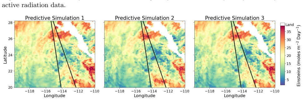
- In the two real data applications, the adjusted posteriors are wider than the unadjusted debiased Whittle posteriors and differ in location from the standard Whittle posteriors, changing the practical conclusions about the spatial range and amplitude.
Reading between the lines
- The same curvature adjustment should transfer directly to one-dimensional time series, where the debiased Whittle likelihood with this calibration could provide well-calibrated Bayesian credible intervals for short series; the paper lists this direction but does not test it.
- A cheap practical safeguard is to run the paper's own coverage check on a handful of prior draws before a full analysis, letting users verify that the Monte Carlo sample size used to build the adjustment is large enough; the paper only partially probes this sensitivity.
- Because the adjustment is built from the point estimate of the parameters and the observed Fisher information, the calibrated posterior is data-dependent in a stronger sense than an ordinary likelihood posterior; this suggests re-running the coverage check whenever the dataset, grid geometry, or prior changes substantially.
Editorial analysis
A structured set of objections, weighed in public.
Referee Report
Summary. The paper proposes two Monte Carlo-based curvature adjustments, C1 and C2, of the debiased spatial Whittle likelihood for Bayesian inference on large stationary random fields. The adjustments follow Ribatet et al. (2012): they rescale the debiased Whittle posterior so that its asymptotic covariance matches the sandwich covariance of the debiased Whittle maximum likelihood estimator. C1 estimates the score covariance J and uses the analytic Hessian H; C2 directly estimates the sampling distribution of the estimator and uses the observed Fisher information. The method is validated in simulation studies with square grids of increasing size, a PC prior, and an irregular domain, using the Monahan-Boos/Cook et al. posterior-quantile checks, and it is applied to sea surface temperature and PAR data. The central claim is that the adjusted posteriors are well-calibrated as measured by coverage properties of credible sets while retaining O(n log n) computation.
Significance. Scalable Bayesian inference for spatial covariance parameters is an area of active interest, and the paper offers a practical solution that combines the debiased Whittle likelihood with composite-likelihood calibration. The Monte Carlo estimation of the sandwich matrix is a reasonable parametric-bootstrap approach and avoids the intractable direct computation of the score variance. The simulation evidence for marginal calibration on large square grids is strong, and the two data applications demonstrate that the method handles missing values and moderately large grids. The paper also gives useful practical guidance on when to prefer C1 over C2. However, the headline calibration claim is only partially supported: the validation is marginal rather than joint, and one simulation setting explicitly shows residual miscalibration in the irregular-domain case. If joint calibration is established or the claims are appropriately qualified, the contribution would be a useful addition to the spatial statistics literature.
major comments (3)
- [3.5, Eq. (26), Figures 3–5] The calibration validation is marginal only. The statistic U^(i) in Eq. (26) is computed for each scalar component of θ (ρ and σ), and the QQ-plots are componentwise. The abstract and Section 3.1 define validity by coverage of posterior sets K_α(X_s), which for p > 1 are sets in R^p. Marginal posterior quantile calibration is necessary but not sufficient: if C_i correctly inflates marginal variances but leaves the correlation between ρ and σ incorrect, all marginal QQ-plots can look uniform while joint credible sets are systematically miscalibrated. Because the adjustment is matrix-valued and explicitly targets the joint covariance G = H J^{-1} H, the paper should report joint coverage, for example empirical coverage of posterior ellipsoids based on the estimated posterior covariance or a multivariate version of the Monahan-Boos check.
- [3.5, Simulation 2, Figure 4] The authors state that for the irregular France domain, both adjustments are 'indistinguishable from a standard uniform between (0, 0.5)' but that the upper half interval shows more concentration of mass, with ρ worse than σ. This is an explicit deviation from the calibration claim in exactly one of the settings the paper advertises (irregular domains). The abstract's unconditional statement that the adjustment gives 'a well-calibrated Bayesian posterior' should either be supported by an additional correction for irregular domains, restricted to the settings where calibration is demonstrated, or accompanied by diagnostics (e.g., larger K, larger M, or alternative domain shapes) showing that the deviation is Monte Carlo noise rather than a systematic effect.
- [3.2, Eq. (17); Conclusion] The theoretical basis for the adjustment is not established for this setting. Equation (17) is imported from composite-likelihood Bernstein-von Mises theory (Ribatet et al., 2012; Kleijn and van der Vaart, 2012). For the spatial debiased Whittle likelihood, the summands in Eq. (8) are not independent: periodogram ordinates at Fourier frequencies are correlated at finite n, and the asymptotic efficiency result for the MdWLE in Guillaumin et al. (2022) does not by itself imply the posterior shape in Eq. (17). The paper does not verify Eq. (17) for finite grids except through marginal QQ-plots. Consequently, the conclusion's claim that the adjustments 'asymptotically satisfy the Bernstein Von-Mises theorem' is not supported by the presented theory. The authors should state the regularity conditions under which Eq. (17) holds for the debiased Whittle likelihood, cite a theorem that covers dependent data, or weaken the theoretical claim and present the method as an empirically calibrated adjustment.
minor comments (5)
- [3.5] The number K of prior draws used in the Monahan-Boos validation is not reported, and the symbol M is used both for the number of simulated datasets used to estimate the adjustment matrices (Algorithms 1 and 2) and for the number of posterior samples used to estimate U^(i). Please report K and disambiguate the two uses of M.
- [4.1] There is a contradiction: the text says the C1 adjustment cannot be applied because it requires derivatives of the Matérn covariance, but then states 'We simulate M = 500 datasets to compute the adjustment C1 matrix.' This should presumably refer to C2.
- [3.4, last paragraph] The text says the PC prior is 'described in more detail in Section 3'; the prior is actually described in Section 3.5 (Simulation 3). The cross-reference should be corrected.
- [3.3, Eq. (24)] Equation (24) appears to contain a typographical bracket: 'fM_A^T fM_A = [G(θ), cM^T cM = H(θ)' presumably should read 'fM_A^T fM_A = G(θ)' and 'cM^T cM = H(θ)'.
- [4.2 and Figure 11] There are typos in Section 4.2 ('Similiar', 'which it the conditional normal density'), and Figure 11 uses iterations 3000, 6000, and 9000; the caption should clarify whether these are thinned MCMC iterations or consecutive draws after burn-in.
Circularity Check
No circularity: the calibration construction does not feed its own coverage target back into the fit, and the headline claim rests on external simulation benchmarks.
full rationale
The paper's derivation chain is self-contained rather than circular. The adjusted likelihood (25) is the Ribatet et al. (2012) composite-likelihood curvature adjustment applied to the debiased Whittle likelihood, and the correction matrices are estimated by parametric bootstrap at the debiased Whittle estimator. The claimed calibration is then checked by the Monahan-Boos / Cook et al. posterior-quantile procedure (26), which is an external benchmark comparing U^(i) to Uniform(0,1) on simulated data drawn from the prior. The coverage target is not used as an input to the construction of C1 or C2: the sandwich quantities H, J and Var[\hat\theta_dW] are estimated from simulated data or analytical gradients, not from the coverage statistic U. The asymptotic justification is imported from Ribatet et al. (2012) and Kleijn and van der Vaart (2012), both external to this paper's authors. The one self-citation, Guillaumin et al. (2022), supplies the debiased Whittle likelihood and the asymptotic variance of its estimator; that is a published theorem with proofs and independent simulation, and the present paper's contribution is the Bayesian calibration, not the debiased Whittle estimator itself. Thus no load-bearing step reduces by construction to its own inputs. A separate completeness concern, that only marginal posterior quantiles are reported rather than joint credible-set coverage, is a validation gap and not a circularity.
Assumptions & free parameters
free parameters (2)
- Monte Carlo sample size M =
M=250, 500, 1000
- Nugget variance σ²ε =
1e-10 (SST), 0.001 (PAR)
assumptions (4)
- ad hoc to paper The composite posterior is approximately N(θ0, |n|^{-1}H^{-1}) (Eq. 17)
- domain assumption The debiased Whittle likelihood is a valid composite likelihood with H ≠ J
- domain assumption Stationarity and square-summable covariance
- ad hoc to paper Monte Carlo estimates of J and G converge quickly enough with M
Cite this review
Pith. "Pith review of Calibrated Bayesian inference for random fields on large irregular domains using the debiased spatial Whittle likelihood." pith.science (2026). https://pith.science/paper/XYVEES4Q
@misc{pith2026250523330,
  author       = {Pith},
  title        = {Pith review of: Calibrated Bayesian inference for random fields on large irregular domains using the debiased spatial Whittle likelihood},
  year         = {2026},
  howpublished = {\url{https://pith.science/paper/XYVEES4Q}},
  note         = {Machine review of arXiv:2505.23330}
}
abstract
Bayesian inference for stationary random fields is computationally demanding. Whittle-type likelihoods in the frequency domain based on the fast Fourier Transform (FFT) have several appealing features: i) low computational complexity of only $\mathcal{O}(n \log n)$, where $n$ is the number of spatial locations, ii) robustness to assumptions of the data-generating process, iii) ability to handle missing data and irregularly spaced domains, and iv) flexibility in modelling the covariance function via the spectral density directly in the spectral domain. It is well known, however, that the Whittle likelihood suffers from bias and low efficiency for spatial data. The debiased Whittle likelihood is a recently proposed alternative with better frequentist properties. We propose a methodology for Bayesian inference for stationary random fields using the debiased spatial Whittle likelihood, with an adjustment from the composite likelihood literature. The adjustment is shown to give a well-calibrated Bayesian posterior as measured by coverage properties of credible sets, without sacrificing the quasi-linear computation time. We apply the method to simulated data and two real datasets.
Figures


Figures from the paper (8 more)


Reference graph
Works this paper leans on
-
[1]
Akaike, H. (1973). Block Toeplitz matrix inversion . SIAM Journal on Applied Mathematics , 24(2):234--241
work page 1973
-
[2]
Anitescu, M., Chen, J., and Stein, M. L. (2017). An inversion-free estimating equations approach for G aussian process models. Journal of Computational and Graphical Statistics , 26(1):98--107
work page 2017
-
[3]
Berliner, L. M., Wikle, C. K., and Cressie, N. (2000). Long-lead prediction of Pacific SSTs via Bayesian dynamic modeling . Journal of Climate , 13(22):3953--3968
work page 2000
-
[4]
Best, N. G., Ickstadt, K., Wolpert, R. L., and Briggs, D. J. (2001). Combining models of health and exposure data: the SAVIAH study. In Spatial Epidemiology: Methods and Applications . Oxford University Press
work page 2001
-
[5]
and Gaetan, C
Bevilacqua, M. and Gaetan, C. (2015). Comparing composite likelihood methods based on pairs for spatial G aussian random fields. Statistics and Computing , 25:877--892
2015
-
[6]
Brockwell, P. J. and Davis, R. A. (2009). Time Series: Theory and Methods . Springer Science & Business Media
work page 2009
-
[7]
Cook, S. R., Gelman, A., and Rubin, D. B. (2006). Validation of software for Bayesian models using posterior quantiles . Journal of Computational and Graphical Statistics , 15(3):675--692
work page 2006
-
[8]
Cressie, N. (1989). Geostatistics. The American Statistician , 43(4):197--202
work page 1989
Show all 53 references
-
[9]
and K \"u nsch, H
Dahlhaus, R. and K \"u nsch, H. (1987). Edge effects and efficient parameter estimation for stationary random fields. Biometrika , 74(4):877--882
1987
-
[10]
and Han, Z
De Oliveira, V. and Han, Z. (2022). On information about covariance parameters in Gaussian M \'a tern random fields . Journal of Agricultural, Biological and Environmental Statistics , 27(4):690--712
2022
-
[11]
Dietrich, C. R. and Newsam, G. N. (1997). Fast and exact simulation of stationary Gaussian processes through circulant embedding of the covariance matrix . SIAM Journal on Scientific Computing , 18(4):1088--1107
1997
-
[12]
T., Drovandi, C., and Kohn, R
Frazier, D. T., Drovandi, C., and Kohn, R. (2023). Calibrated generalized B ayesian inference. arXiv preprint arXiv:2311.15485
2023
-
[13]
Fuentes, M. (2007). Approximate likelihood for large irregularly spaced spatial data. Journal of the American Statistical Association , 102(477):321--331
2007
-
[14]
Fuglstad, G.-A., Simpson, D., Lindgren, F., and Rue, H. (2019). Constructing priors that penalize the complexity of G aussian random fields. Journal of the American Statistical Association , 114(525):445--452
2019
-
[15]
E., Diggle, P., Guttorp, P., and Fuentes, M
Gelfand, A. E., Diggle, P., Guttorp, P., and Fuentes, M. (2010). Handbook of Spatial Statistics . CRC press
2010
-
[16]
J., Marin, O., Schanen, M., and Stein, M
Geoga, C. J., Marin, O., Schanen, M., and Stein, M. L. (2023). Fitting Mat \'e rn smoothness parameters using automatic differentiation . Statistics and Computing , 33(2):48
2023
-
[17]
P., Sykulski, A
Guillaumin, A. P., Sykulski, A. M., Olhede, S. C., and Simons, F. J. (2022). The debiased spatial W hittle likelihood. Journal of the Royal Statistical Society Series B: Statistical Methodology , 84(4):1526--1557
2022
-
[18]
Guilleminot, J. (2020). Modeling non-Gaussian random fields of material properties in multiscale mechanics of materials . In Uncertainty Quantification in Multiscale Materials Modeling , pages 385--420. Woodhead Publishing
2020
-
[19]
and Fuentes, M
Guinness, J. and Fuentes, M. (2017). Circulant embedding of approximate covariances for inference from G aussian data on large lattices. Journal of Computational and Graphical Statistics , 26(1):88--97
2017
-
[20]
Guyon, X. (1982). Parameter estimation for a stationary process on a d-dimensional lattice. Biometrika , 69(1):95--105
1982
-
[21]
Heyde, C. C. (1997). Quasi-Likelihood and its Application: A General Approach to Optimal Parameter Estimation . Springer
1997
-
[22]
and Cressie, N
Hrafnkelsson, B. and Cressie, N. (2003). Hierarchical modeling of count data with application to nuclear fall-out. Environmental and Ecological Statistics , 10:179--200
2003
-
[23]
and Guinness, J
Katzfuss, M. and Guinness, J. (2021). A general framework for V ecchia approximations of G aussian processes. Statistical Science , 36(1):124 -- 141
2021
-
[24]
Kent, J. T. and Mardia, K. V. (1996). Spectral and circulant approximations to the likelihood for stationary Gaussian random fields . Journal of Statistical Planning and Inference , 50(3):379--394
1996
-
[25]
and van der Vaart, A
Kleijn, B. and van der Vaart, A. (2012). The Bernstein-Von-Mises theorem under misspecification . Electronic Journal of Statistics , 6:354--381
2012
-
[26]
Körner, T. W. (1988). Fourier Analysis . Cambridge University Press
1988
-
[27]
Lindgren, F., Rue, H., and Lindstr \"o m, J. (2011). An explicit link between G aussian fields and G aussian M arkov random fields: the stochastic partial differential equation approach. Journal of the Royal Statistical Society: Series B (Statistical Methodology) , 73(4):423--498
2011
-
[28]
Matheron, G. (1963). Principles of geostatistics. Economic Geology , 58(8):1246--1266
1963
-
[29]
and Yajima, Y
Matsuda, Y. and Yajima, Y. (2009). Fourier analysis of irregularly spaced data on R^d . Journal of the Royal Statistical Society Series B: Statistical Methodology , 71(1):191--217
2009
-
[30]
H., Kim, S., B \"u rkner, P., Huurre, N., Faltejskov \'a , K., Gelman, A., and Vehtari, A
Modr \'a k, M., Moon, A. H., Kim, S., B \"u rkner, P., Huurre, N., Faltejskov \'a , K., Gelman, A., and Vehtari, A. (2023). Simulation-based calibration checking for Bayesian computation: The choice of test quantities shapes sensitivity . Bayesian Analysis , 1(1):1--28
2023
-
[31]
Monahan, J. F. and Boos, D. D. (1992). Proper likelihoods for Bayesian analysis . Biometrika , 79(2):271--278
1992
-
[32]
Parzen, E. (1963). On spectral analysis with missing observations and amplitude modulation. Sankhyā: The Indian Journal of Statistics, Series A (1961-2002) , 25(4):383--392
1963
-
[33]
Percival, D. B. and Walden, A. T. (1993). Spectral Analysis for Physical Applications . Cambridge University Press
1993
-
[34]
Quiroz, M., Kohn, R., Villani, M., and Tran, M.-N. (2019). Speeding up MCMC by efficient data subsampling . Journal of the American Statistical Association , 114(526):831--843
2019
-
[35]
Quiroz, M., Tran, M.-N., Villani, M., Kohn, R., and Dang, K.-D. (2021). The block- P oisson estimator for optimally tuned exact subsampling MCMC . Journal of Computational and Graphical Statistics , 30(4):877--888
2021
-
[36]
Rasmussen, C. E. and Williams, C. K. (2006). Gaussian Processes for Machine Learning . MIT Press Cambridge, MA
2006
-
[37]
Ribatet, M., Cooley, D., and Davison, A. C. (2012). Bayesian inference from composite likelihoods, with an application to spatial extremes. Statistica Sinica , 22(2):813--845
2012
-
[38]
and Held, L
Rue, H. and Held, L. (2005). Gaussian Markov Random Fields: Theory and Applications . Chapman and Hall/CRC
2005
-
[39]
Salomone, R., Quiroz, M., Kohn, R., Villani, M., and Tran, M.-N. (2020). Spectral subsampling MCMC for stationary time series . In International Conference on Machine Learning , pages 8449--8458. PMLR
2020
-
[40]
and Wu, W
Shao, X. and Wu, W. B. (2007). Asymptotic spectral theory for nonlinear time series. The Annals of Statistics , 35(4):1773--1801
2007
-
[41]
Sid \'e n, P., Lindgren, F., Bolin, D., Eklund, A., and Villani, M. (2021). Spatial 3D Mat \'e rn priors for fast whole-brain fMRI analysis. Bayesian Analysis , 16(4):1251--1278
2021
-
[42]
Simons, F. J. and Olhede, S. C. (2013). Maximum-likelihood estimation of lithospheric flexural rigidity, initial-loading fraction and load correlation, under isotropy. Geophysical Journal International , 193(3):1300--1342
2013
-
[43]
Sowell, F. (1989). A decomposition of block T oeplitz matrices with applications to vector time series. Unpublished manuscript available at https://www.researchgate.net/profile/Fallaw-Sowell
1989
-
[44]
L., Chen, J., and Anitescu, M
Stein, M. L., Chen, J., and Anitescu, M. (2013). Stochastic approximation of score function for G aussian procceses. The Annals of Applied Statistics , 7:1162--1191
2013
-
[45]
R., Stein, M
Stroud, J. R., Stein, M. L., and Lysen, S. (2017). Bayesian and maximum likelihood estimation for G aussian processes on an incomplete lattice. Journal of Computational and Graphical Statistics , 26(1):108--120
2017
-
[46]
M., Olhede, S
Sykulski, A. M., Olhede, S. C., Guillaumin, A. P., Lilly, J. M., and Early, J. J. (2019). The debiased whittle likelihood. Biometrika , 106(2):251--266
2019
-
[47]
E., Mulholland, J
Tolbert, P. E., Mulholland, J. A., Macintosh, D. L., Xu, F., Daniels, D., Devine, O. J., Carlin, B. P., Klein, M., Butler, A. J., Nordenberg, D. F., et al. (2000). Air quality and pediatric emergency room visits for asthma and Atlanta, Georgia . American Journal of Epidemiolog...
2000
-
[48]
Van der Vaart, A. W. (2000). Asymptotic Statistics . Cambridge University Press
2000
-
[49]
Varin, C., Reid, N., and Firth, D. (2011). An overview of composite likelihood methods. Statistica Sinica , 21:5--42
2011
-
[50]
Vecchia, A. V. (1988). Estimation and model identification for continuous spatial processes. Journal of the Royal Statistical Society: Series B (Methodological) , 50(2):297--312
1988
-
[51]
Villani, M., Quiroz, M., Kohn, R., and Salomone, R. (2024). Spectral subsampling MCMC for stationary multivariate time series with applications to vector ARTFIMA processes. Econometrics and Statistics , 32:98--121
2024
-
[52]
White, H. (1982). Maximum likelihood estimation of misspecified models. Econometrica , 50(1):1--25
1982
-
[53]
Whittle, P. (1954). On stationary processes in the plane. Biometrika , 41:434--449
1954
Reviewed August 7, 2026 · model on record in the stance chip above.
Discussion (0). Sign in to comment.