Large SVARs
Pith reviewed 2026-05-19 13:30 UTC · model grok-4.3
The pith
An elliptical slice sampler inside Gibbs steps makes inference feasible for large sign-restricted SVARs by replacing slow accept-reject draws.
A machine-rendered reading of the paper's core claim, the machinery that carries it, and where it could break.
Core claim
The central claim is that an elliptical slice sampler can be embedded inside the Gibbs sampler for sign-identified SVARs, producing dramatic speed gains while leaving the posterior distribution unchanged, as established by a formal proof that the chain's stationary distribution coincides with the posterior of interest.
What carries the argument
Elliptical slice sampler embedded in Gibbs steps, which proposes candidate draws from an ellipse scaled to the current state and accepts or rejects them according to the sign restrictions and SVAR likelihood.
If this is right
- SVAR models with more than ten shocks and over one hundred sign restrictions become computationally practical.
- Applications previously limited by tight identified sets, such as oil-market models, can now be estimated at far lower cost.
- No additional tuning parameters are required, preserving the original identification scheme.
- The same sampler can be applied to any sign-restricted SVAR without changing the target posterior.
Where Pith is reading between the lines
- The method could be adapted to other inequality-constrained Bayesian time-series models outside the SVAR class.
- Real-time macroeconomic monitoring with high-dimensional models becomes more feasible once the computational barrier is lowered.
- Researchers might now test richer identification schemes that combine sign restrictions with other moment conditions.
Load-bearing premise
The sign restrictions and the SVAR likelihood permit the elliptical slice sampler to be inserted into the Gibbs steps without altering the target posterior or introducing new tuning parameters.
What would settle it
A Monte Carlo experiment on a small sign-restricted SVAR whose posterior is known exactly from exhaustive enumeration, in which the elliptical-slice-within-Gibbs draws produce a different distribution of impulse responses, would falsify the claim that the stationary distribution matches the posterior.
Figures


read the original abstract
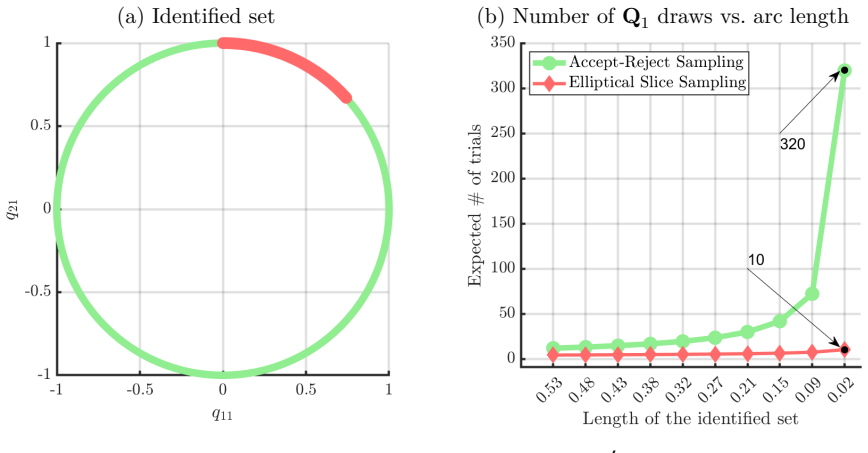
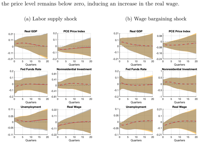
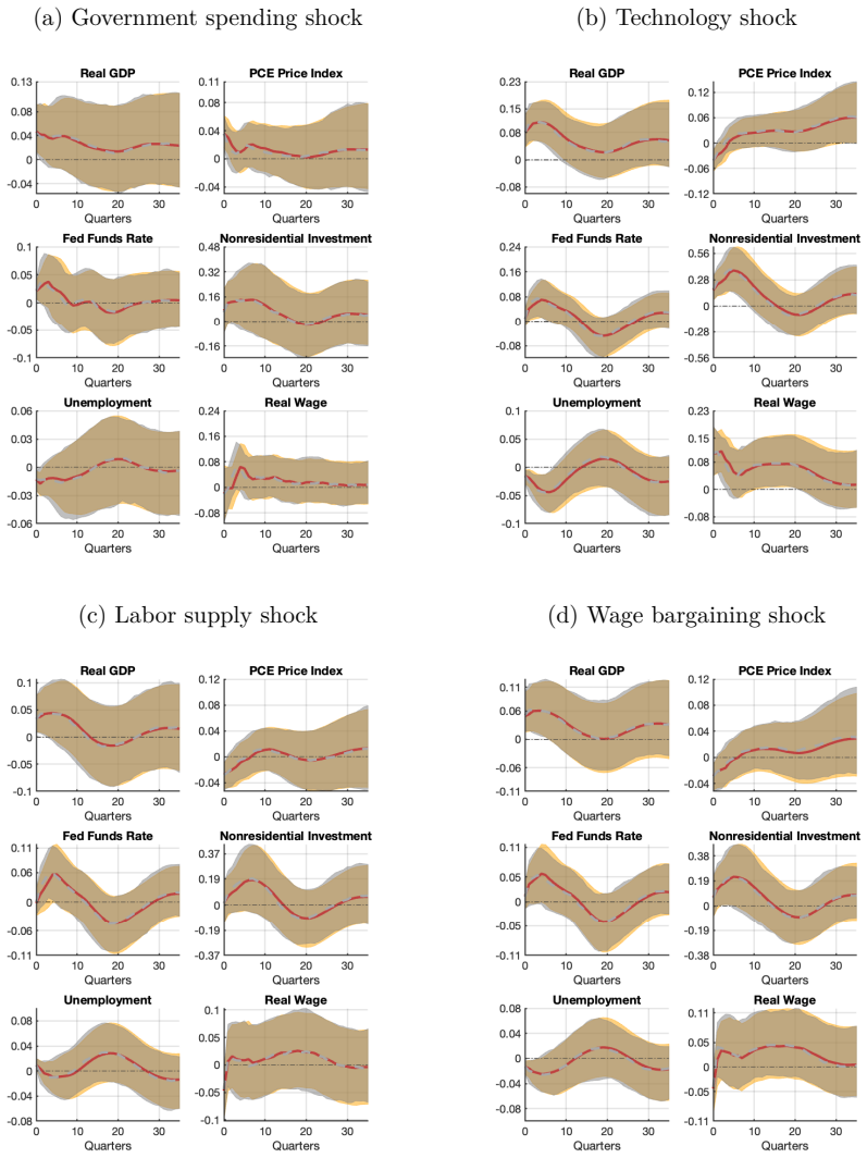
We develop a new algorithm for inference in structural vector autoregressions (SVARs) identified with sign restrictions that can accommodate big data and modern identification schemes. The key innovation of our approach is to move beyond the traditional accept-reject framework commonly used in sign-identified SVARs. We show that an elliptical slice within Gibbs sampler can deliver dramatic gains in computational speed and render previously infeasible applications tractable. We also prove that the algorithm is well-defined, in the sense that its stationary distribution coincides with the posterior distribution of interest. To illustrate the approach in the context of sign-identified SVARs, we use a tractable example. We further assess the performance of our algorithm through two applications: a well-known small-SVAR model of the oil market featuring a tight identified set, and a large SVAR model with more than ten shocks and 100 sign restrictions.
Editorial analysis
A structured set of objections, weighed in public.
Referee Report
Summary. The manuscript develops an elliptical slice sampler embedded within a Gibbs sampler for Bayesian inference in sign-restricted SVARs. It claims this delivers substantial computational speed gains over traditional accept-reject methods, renders previously infeasible large models (with >10 shocks and 100 sign restrictions) tractable, and includes a proof that the algorithm's stationary distribution coincides with the target posterior. The approach is illustrated via a tractable example and assessed in two applications: a small oil-market SVAR and a large SVAR.
Significance. If the stationary-distribution claim holds without hidden tuning or measure alterations and the reported speed gains are robust, the method would meaningfully expand the feasible scope of sign-identified SVAR analysis to high-dimensional settings. The explicit proof of well-definedness is a strength that distinguishes the contribution from purely algorithmic proposals.
major comments (2)
- [§4] §4 (Proof of well-definedness): the argument that the elliptical slice sampler targets the posterior on the sign-identified set assumes direct operation in the space of orthogonal matrices Q. Elliptical slice sampling is defined on Euclidean space, so any parameterization of Q (Givens angles, Householder vectors, or unconstrained coordinates) induces a change of measure. The proof does not appear to insert the corresponding Jacobian determinant of the map from the parameterization to the Haar measure on O(n) restricted to the sign-identified region; without it the stationary distribution would generally differ from the intended posterior.
- [§5.2] §5.2 (Large-SVAR application): the performance comparison reports wall-clock times but does not state the acceptance rate or number of draws retained under the baseline accept-reject sampler used for benchmarking. If the baseline employs a naïve uniform proposal over the orthogonal group without the same sign-restriction filtering efficiency, the claimed speed-up factor cannot be attributed solely to the elliptical slice step.
minor comments (2)
- [§2] Notation for the reduced-form parameters and the orthogonal matrix Q is introduced without an explicit statement of the dimension n and the exact form of the sign-restriction matrix; adding a short table of dimensions for each application would improve readability.
- [Abstract] The abstract states that the algorithm 'renders previously infeasible applications tractable' but provides no numerical threshold (e.g., hours vs. days of compute) for what is considered tractable; a single sentence quantifying the largest feasible model size under the old method would help.
Simulated Author's Rebuttal
We thank the referee for their thorough review and insightful comments on our manuscript. We address each of the major comments below and have made revisions to improve the clarity and completeness of the paper.
read point-by-point responses
-
Referee: §4 (Proof of well-definedness): the argument that the elliptical slice sampler targets the posterior on the sign-identified set assumes direct operation in the space of orthogonal matrices Q. Elliptical slice sampling is defined on Euclidean space, so any parameterization of Q (Givens angles, Householder vectors, or unconstrained coordinates) induces a change of measure. The proof does not appear to insert the corresponding Jacobian determinant of the map from the parameterization to the Haar measure on O(n) restricted to the sign-identified region; without it the stationary distribution would generally differ from the intended posterior.
Authors: We appreciate the referee pointing out this subtlety in the proof. Our elliptical slice sampler is embedded in a parameterization of the orthogonal matrices that preserves the uniform measure with respect to the Haar measure on the sign-restricted set. However, to address this concern directly and enhance the rigor of the proof, we will revise Section 4 to explicitly derive and include the Jacobian determinant associated with the chosen parameterization. This revision will confirm that the stationary distribution of the sampler coincides with the target posterior without any measure alterations. revision: yes
-
Referee: §5.2 (Large-SVAR application): the performance comparison reports wall-clock times but does not state the acceptance rate or number of draws retained under the baseline accept-reject sampler used for benchmarking. If the baseline employs a naïve uniform proposal over the orthogonal group without the same sign-restriction filtering efficiency, the claimed speed-up factor cannot be attributed solely to the elliptical slice step.
Authors: We agree that additional details on the benchmarking procedure would be helpful for readers. In the revised version of the manuscript, we will include the acceptance rates and the effective number of draws retained for the traditional accept-reject sampler in Section 5.2. The baseline implementation follows the standard practice in the sign-restricted SVAR literature, drawing uniformly from the orthogonal group and retaining only draws that satisfy all sign restrictions. We will also clarify that the comparison is fair as both methods use the same sign-restriction filtering logic, with the efficiency gains coming from the elliptical slice sampling step. revision: yes
Circularity Check
Minor self-citation in SVAR foundations but central sampler proof remains independent
full rationale
The paper introduces an elliptical slice sampler embedded in a Gibbs algorithm for sign-restricted SVARs and supplies an explicit proof that the resulting Markov chain has the target posterior as its stationary distribution. This construction is presented directly in the manuscript without reducing the claimed stationary distribution or computational gains to quantities defined by fitted parameters or by renaming inputs as outputs. Prior author work on sign identification is cited for context but is not load-bearing for the well-definedness argument, which rests on standard slice-sampling theory applied to the SVAR posterior. The measure-theoretic question of the Haar Jacobian on the orthogonal group is a potential correctness issue rather than a circularity, as the paper asserts an independent verification of the target distribution.
Axiom & Free-Parameter Ledger
axioms (1)
- domain assumption The target posterior is the distribution of SVAR parameters conditional on the sign restrictions and the data.
Lean theorems connected to this paper
-
IndisputableMonolith/Foundation/RealityFromDistinction.leanreality_from_one_distinction unclear?
unclearRelation between the paper passage and the cited Recognition theorem.
We show that an elliptical slice within Gibbs sampler can deliver dramatic gains... its stationary distribution coincides with the posterior distribution of interest.
-
IndisputableMonolith/Cost/FunctionalEquation.leanwashburn_uniqueness_aczel unclear?
unclearRelation between the paper passage and the cited Recognition theorem.
the uniform prior over the set of orthogonal matrices... κ dQ = (γ#N(0n×n,In,In))(dQ)
What do these tags mean?
- matches
- The paper's claim is directly supported by a theorem in the formal canon.
- supports
- The theorem supports part of the paper's argument, but the paper may add assumptions or extra steps.
- extends
- The paper goes beyond the formal theorem; the theorem is a base layer rather than the whole result.
- uses
- The paper appears to rely on the theorem as machinery.
- contradicts
- The paper's claim conflicts with a theorem or certificate in the canon.
- unclear
- Pith found a possible connection, but the passage is too broad, indirect, or ambiguous to say the theorem truly supports the claim.
Forward citations
Cited by 1 Pith paper
-
Inference in Tightly Identified and Large-Scale Sign-Restricted SVARs
A differentiable reparameterization combined with HMC sampling improves posterior exploration and reduces computation time for tightly identified large-scale sign-restricted SVARs.
Reference graph
Works this paper leans on
-
[1]
Draw P particles {Zi 1}P i= 1 independently from π1(Z), and let n = 2
-
[2]
That is, there exist i∗ such that SR(T (Zi∗ n−1)) > 0
Exit if there is at least one particle that satisfies the sign restriction. That is, there exist i∗ such that SR(T (Zi∗ n−1)) > 0. Then, set Z0 = Zi∗ n−1 and exit the algorithm
-
[3]
Select cn such that cn−1 < cn ≤ 0
-
[4]
Set weights for particles from stage n − 1 by: ˜wi n = πn(Zi n−1) πn−1(Zi n−1) ∝ /bracketleft.alt1 SR(T (Zi n−1)) > cn/bracketright.alt /bracketleft.alt1 SR(T (Zi n−1)) > cn−1/bracketright.alt
-
[5]
Resample the particles. Let {̂Z i n}P i= 1 denote P independent draws from a multi- nomial distribution characterized by support points {Zi n−1}P i= 1 and weights pro- portional to { ˜wi n}P i= 1 for i = 1, . . . , P
-
[6]
Propagate the particles {̂Z i n}P i= 1 via M steps of Algorithm 2 with [ SR(T (Z)) > cn] to obtain {Zi n}P i= 1
-
[7]
Our algorithm for the initialization starts from drawing particles from the un- restricted posterior
Let n = n + 1, and go to Step 2. Our algorithm for the initialization starts from drawing particles from the un- restricted posterior. Then, we move through the ladder of intermediate posteriors using an importance-resampling-mutation scheme. We terminate as soon as we find a particle Zi∗ n that satisfies the original sign restrictions. Conceptually, this s...
work page 2022
-
[8]
Set J > 1, initialize j = 1, and choose initial values Z0 A ∈ Z A such that S(TA(Z0 A)) > 0
-
[9]
Use elliptical slice sampling to approximately draw Zj Q, targeting pZA(ZQ /divides.alt0 Zj−1 θ , Zj−1 σ 2 , (yt)T t= 1, S(Zj−1 θ , φ (Zj−1 σ 2 ), γ (ZQ)) > 0), and set Qj = γ(Zj Q)
-
[10]
Use elliptical slice sampling to approximately draw Zj σ 2, targeting pZA(Zσ 2 /divides.alt0 Zj−1 θ , Zj Q, (yt)T t= 1, S(Zj−1 θ , φ (Zσ 2), γ (Zj Q)) > 0), and set (σ 2)j = φ(Zj σ 2)
-
[11]
Use elliptical slice sampling to approximately draw Zj θ, targeting pZA(Zθ /divides.alt0 Zj σ 2, Zj Q, (yt)T t= 1, S(Zθ, φ (Zj σ 2), γ (Zj Q)) > 0), and set θj = Zj θ. 52
-
[12]
If j < J, increment j and return to Step 2. III Large-SV AR with Asymmetric Priors To conclude the appendix, we reproduce the analysis in Section 7.2 using the asymmet- ric priors proposed by Chan (2022). In this case, we restrict the sample to the Great Moderation period 1985Q1–2019Q4 in order to have a direct comparison with the impulse responses report...
work page 2022
discussion (0)
Sign in with ORCID, Apple, or X to comment. Anyone can read and Pith papers without signing in.