REVIEW 3 major objections 4 minor 37 references
Bayesian kernel machine regression for heteroscedastic health outcome data
T0 review · 3 major / 4 minor · reviewed 2026-08-07 · deepseek-v4-flash
Pith's one-line read The paper claims that adding a per-person error-variance model to Bayesian kernel machine regression improves mixture effect estimates and narrows credible intervals in two child metal-exposure studies.
desk verdict Useful and mathematically sound heteroscedastic BKMR extension, but the reported WAIC gains and narrower intervals are likely inflated by post-hoc selection of variance covariates and lack simulation support. read the letter →
The pith
A machine-rendered reading of the paper's core claim, the machinery that carries it, and where it could break.
The reading
What carries the argument
The load-bearing object is the variance model $\log(\sigma_i^2)=w_i'\gamma$, where $w_i$ selects individual characteristics (or just an intercept) and $\gamma$ are regression coefficients; it is assembled into the diagonal matrix $S_\gamma$ whose $i$th diagonal entry is $\exp(w_i'\gamma)$. Because the exposure function $h$ is integrated out, the likelihood becomes multivariate normal with covariance $\tau K_r + S_\gamma$, so the existing BKMR machinery for cross-sections and predictions carries over with the covariance term modified. The diagnostic function uses Bayesian residuals—the observed outcome minus the posterior mean of $h(z_i)+x_i'\beta$—plotted against fitted values and predictors, to indicate which variables belong in $W$. The paper's comparisons rely on the widely applicable information criterion (WAIC) and on credible-interval widths for the same exposure-response cross-sections under both models.
What would settle it
A direct falsifier is a simulation study in which outcomes are generated from a heteroscedastic mixture model with known variance covariates: if, over many replicates, the 95% credible intervals for the exposure-response curve cover the truth less than 95% of the time, or if fixing the variance covariates in advance (rather than selecting them from the data) erases most of the reported fit advantage of HBKMR over BKMR, the central claim would be contradicted.
Extended reading notes
Core claim
On its own terms, the paper's central claim is that specifying a Bayesian hierarchical variance model for the error term, $\log(\sigma_i^2)=w_i'\gamma$ with $S_\gamma=\mathrm{diag}(\exp(w_i'\gamma))$, turns standard BKMR into a model that remains estimable in closed form after integrating out the exposure function $h$: $y \mid \beta,\tau,r,\gamma \sim \mathrm{MVN}(X\beta,\ \tau K_r + S_\gamma)$. Posterior draws of $(\beta,\tau,r,\gamma)$ then feed conditional multivariate normal formulas for exposure-response cross-sections such as $h(z_{0.75})-h(z_{0.50})$, and for predictive intervals, both with the heteroscedastic correction included. The paper further claims that the standard model is the special case $w_i=1$, so the two are directly comparable, and that in the two case studies the variance-model extension produces WAIC improvements of 29–97 points, typically narrower credible intervals, and prediction intervals that widen for subgroups with genuinely higher residual variability, such as children from a specific district or younger children.
Load-bearing premise
The load-bearing premise is that picking the variance-model variables by looking at the same data used to measure improvement does not inflate the apparent gains, which the paper does not test with simulations.
Editorial extensions
If this is right
- Researchers using standard BKMR should first run residual diagnostics; when variance changes with a covariate, point estimates can shift and credible intervals can become materially narrower after correction.
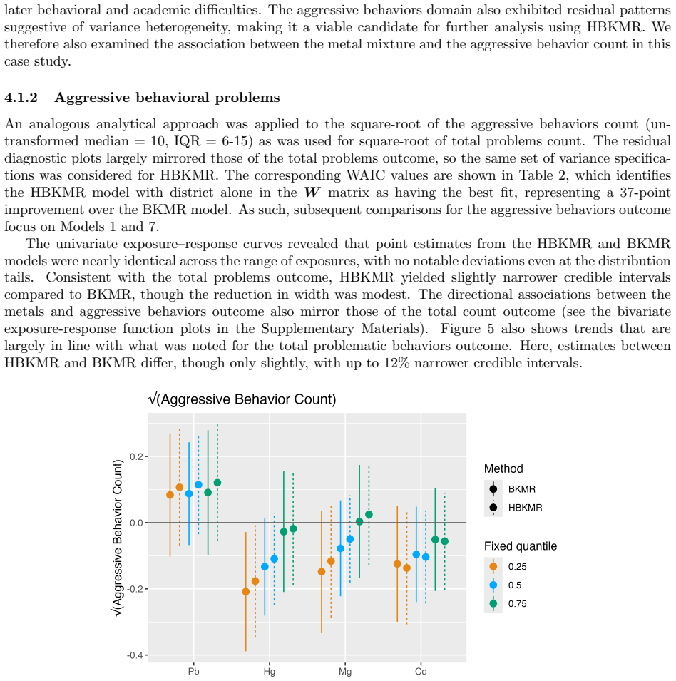
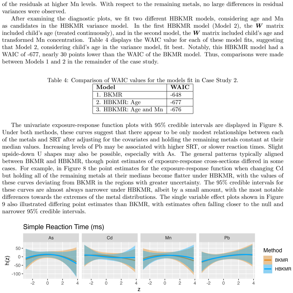
- In the two case studies, accounting for heteroscedasticity reduced credible-interval widths by roughly 6 to 20 percent, so conclusions about which metals drive an effect and how precisely they are estimated can depend on the variance model.
- HBKMR produces prediction intervals that widen for identifiable subgroups with higher residual variance, which is more honest than constant-variance intervals for individual-level prediction and for causal-effect estimates built from counterfactual outcomes.
- Because HBKMR reduces to BKMR when the variance model contains only an intercept, adopting it costs nothing when no heteroscedasticity is present and only adds parameters when the diagnostics justify them.
- The diagnostic plots can also hint at whether the chosen Gaussian kernel is appropriate, extending the value of model checking beyond the variance assumption.
Reading between the lines
- An implication the authors leave implicit is that the reported fit gains may be optimistic: the variance covariates were chosen from residual plots and WAIC comparisons on the same datasets used to report improvement, and no simulation study tests how often this selection procedure would promote noise.
- A testable extension is to let the variance model be nonlinear, for example letting $\log(\sigma_i^2)$ depend on the exposure-response function or on exposure quantiles, which could capture variance structures the linear-in-$w$ model misses.
- The framework also suggests a cheap robustness check for published BKMR analyses: re-fit with a variance model for each covariate that shows residual trends, and if credible intervals narrow substantially, the original intervals were overstating precision.
- Because HBKMR yields subgroup-specific prediction intervals, it could support precision environmental health by flagging children whose high-variance residual profile, not just their high mean outcome, warrants follow-up—a use the paper mentions only briefly.
Editorial analysis
A structured set of objections, weighed in public.
Referee Report
Summary. The paper proposes Heteroscedastic Bayesian Kernel Machine Regression (HBKMR), an extension of BKMR that models the error variance as log(σ_i²) = w_i'γ, thereby relaxing the constant-variance assumption. The authors derive the marginal posterior after integrating out the latent function h, giving y | β, γ, τ, r ~ MVN(Xβ, τK_r + S_γ), and provide conditional distributions for posterior inference on the exposure-response function h_new and on predicted outcomes. They also introduce a residual-based diagnostic function for detecting heteroscedasticity in BKMR fits. The method is illustrated in two case studies—prenatal metal exposure and toddler behavior in Suriname, and metal exposure and reaction time in Kentucky children—where HBKMR is reported to yield WAIC improvements of 29 to 97 points relative to BKMR, along with generally narrower 95% credible intervals. The paper does not include a simulation study.
Significance. If the empirical claims are sustained, the contribution is useful for environmental mixture analyses where heteroscedasticity is present: the model is a natural extension of BKMR, the integration of h is correct and clearly derived in the appendix, and the NIMBLE implementation allows flexible prior specification and direct model comparison. The diagnostic plotting function addresses a genuine gap, as the homoscedasticity assumption is rarely checked in practice. The main significance hinges on whether the reported WAIC improvements reflect genuine predictive gains rather than post-hoc selection of the variance covariates W on the same data used to compute WAIC. As presented, the central empirical evidence is not yet conclusive because no simulation or independent validation study is provided to calibrate the uncertainty estimates or to assess the selection procedure.
major comments (3)
- [§4.1.1 and §4.2] The variance covariates W are selected from the same data used to report the WAIC gains. In Section 4.1.1, Figure 1 is used to propose candidate variance models, and Table 2 then compares six HBKMR fits by WAIC on the same 692 observations; the best model (Pb + district) is reported as a 97-point improvement. Section 4.2 likewise selects age from the diagnostic plots and Table 4 reports a 30-point WAIC improvement over BKMR. Because WAIC is used both to select W and to measure the selected model's performance, the reported WAIC reductions are optimistic estimates of out-of-sample predictive performance; the magnitude of the optimism cannot be assessed without a simulation or a holdout-based evaluation.
- [§3.2 and §4] The paper emphasizes narrower 95% credible intervals under HBKMR as a benefit, but no simulation checks whether these intervals attain nominal coverage. In Section 3.2, credible intervals for h_new are constructed via a normal approximation using E(Σ) and Var(μ); the coverage of this approximation, particularly after selection of W from data, is unverified. Without calibration results, the reported 6–17% reductions in interval width (Section 4.2, Table 5) could reflect underestimation of uncertainty rather than genuine precision gains.
- [§5] The Discussion concedes that 'an in-depth simulation study could uncover settings in which differences in point estimates may be most pronounced.' This is a significant limitation for the central claim because the paper's main evidence is entirely case-study based. The lack of a simulation study also leaves open whether the WAIC differences could be driven by selection overfitting rather than by true heteroscedasticity; a simulation would allow the authors to evaluate the selection procedure's effect on WAIC and on credible interval coverage.
minor comments (4)
- [§2.1] The definition of Bayesian residuals relies on the approximation E(h(zi)|y) computed from posterior means of τ and r, as in Bobb et al. The manuscript would benefit from a brief discussion of the accuracy of this approximation, since the diagnostic plots are used to motivate the variance model.
- [§4.1.1] In Table 2, the row labels for Models 6 and 7 appear reversed in the text: the text says 'the HBKMR model with district and Pb included in the W matrix had the lowest WAIC (2494)' which matches Model 3, but the description of the aggressive outcome analysis selects Model 7 (District) as best; this is internally consistent but the ordering in Table 2 is easy to misread and could be clarified.
- [§3.3] The notation S_γ(W_new) is introduced but the text does not explain how W_new is obtained for new individuals; this is a small clarity issue that could confuse readers implementing prediction.
- [Appendix] In the derivation, the sentence 'which is the kernel of a normal distribution with mean Xβ and covariance matrix S_γ + τK_r' is correct, but the intermediate step using the Woodbury identity would benefit from a one-line explanation for readers not familiar with the identity.
Circularity Check
No circularity by construction: the HBKMR posterior is derived from standard multivariate-normal algebra, and the WAIC improvements rest on a data-driven choice of variance covariates W, an in-sample selection caveat rather than a definitional circularity.
full rationale
The derivation chain is self-contained. Section 3.1 and the Appendix integrate h out of the joint posterior by completing the square, obtaining y | β, γ, τ, r ∼ MVN(Xβ, τKr + Sγ); Sections 3.2 and 3.3 then use the standard multivariate-normal conditioning formulas with the diagonal variance model log(σ²ᵢ) = wᵢ′γ. No estimand is defined in terms of another estimand, and no parameter is fixed to force a result: at Q = 0 the model reduces exactly to BKMR, and this reduction is used only to make the WAIC comparison fair under identical priors. The residual diagnostic (Section 2.1) gives an explicit residual definition and cites Bobb et al. for the approximation of E(h(zᵢ) | y); that is prior external work, not a self-citation, and it does not smuggle in a conclusion. Self-citations (refs 16–18, 30–34) are background or cohort-source citations and are not load-bearing. The one genuine caveat is empirical: the variance covariates W are selected after inspecting the BKMR residual plots (Figures 1 and 7) and comparing WAIC on the same datasets (Tables 2 and 4), and the selected models' 97-point and ~30-point WAIC reductions are then reported as improvements; no simulation checks the coverage of the narrower credible intervals, and Section 5 concedes the absence of an in-depth simulation study. This in-sample selection can bias the apparent gains, but it is a model-selection limitation, not circularity: the WAIC values and interval widths are computed from the fitted posteriors rather than set equal to the selection inputs, the interval narrowing is empirical (some HBKMR predictive intervals are wider, e.g., Nickerie in Figure 6), and none of the enumerated circularity patterns is present with quotable equation-level evidence.
Assumptions & free parameters
free parameters (2)
- gamma (variance model coefficients) =
not reported numerically
- variance model predictor set W =
Case Study 1 Total: Pb and district; Aggressive: district; Case Study 2: child age
assumptions (5)
- standard math MVN conditioning and Woodbury matrix identity are valid for integrating h out of the posterior.
- domain assumption The Gaussian kernel with component weights r adequately captures the exposure-response surface in both cohorts.
- ad hoc to paper Bayesian residuals computed from posterior means of h and beta, with E(h|y) approximated via posterior means of tau and r, correctly reveal heteroscedasticity.
- domain assumption WAIC comparisons on the same data used to select W are a valid basis for claiming improved fit.
- domain assumption A normal approximation to the posterior of hnew cross-sections yields valid 95% credible intervals.
Cite this review
Pith. "Pith review of Bayesian kernel machine regression for heteroscedastic health outcome data." pith.science (2026). https://pith.science/paper/QHI2VMEU
@misc{pith2026250523644,
  author       = {Pith},
  title        = {Pith review of: Bayesian kernel machine regression for heteroscedastic health outcome data},
  year         = {2026},
  howpublished = {\url{https://pith.science/paper/QHI2VMEU}},
  note         = {Machine review of arXiv:2505.23644}
}
read the original abstract
The field of environmental epidemiology has placed an increasing emphasis on understanding the health effects of mixtures of metals, chemicals, and pollutants in recent years. Bayesian Kernel Machine Regression (BKMR) is a statistical method that has gained significant traction in environmental mixture studies due to its ability to account for complex non-linear relationships between the exposures and health outcome and its ability to identify interaction effects between the exposures. However, BKMR makes the crucial assumption that the error terms have a constant variance, and this assumption is not typically checked in practice. In this paper, we create a diagnostic function for checking this constant variance assumption in practice and develop Heteroscedastic BKMR (HBKMR) for environmental mixture analyses where this assumption is not met. By specifying a Bayesian hierarchical variance model for the error term variance parameters, HBKMR produces updated estimates of the environmental mixture's health effects and their corresponding 95% credible intervals. We apply HBKMR in two real-world case studies that motivated this work: 1) Examining the effects of prenatal metal exposures on behavioral problems in toddlers living in Suriname and 2) Assessing the impacts of metal exposures on simple reaction time in children living near coal-fired power plants in Kentucky. In both case studies, HBKMR provides a substantial improvement in model fit compared to BKMR, with differences in some of the mixture effect estimates and typically narrower 95% credible intervals after accounting for the heteroscedasticity.
Figures


Figures from the paper (7 more)





Reference graph
Works this paper leans on
-
[1]
Joubert BR, Kioumourtzoglou MA, Chamberlain T, Chen HY, Gennings C, Turyk ME, et al. Power- ing research through innovative methods for mixtures in epidemiology (PRIME) program: novel and expanded statistical methods. Int J Environ Res Public Health. 2022;19(3):1378. 17
work page 2022
-
[2]
Bayesian ker- nel machine regression for estimating the health effects of multi-pollutant mixtures
Bobb JF, Valeri L, Claus Henn B, Christiani DC, Wright RO, Mazumdar M, et al. Bayesian ker- nel machine regression for estimating the health effects of multi-pollutant mixtures. Biostatistics. 2015;16(3):493-508
work page 2015
-
[3]
Bobb JF, Claus Henn B, Valeri L, Coull BA. Statistical software for analyzing the health effects of multiple concurrent exposures via Bayesian kernel machine regression. Environ Health. 2018;17(1):1-10
work page 2018
-
[4]
Mutiso F, Li H, Pearce JL, Benjamin-Neelon SE, Mueller NT, Neelon B. Bayesian kernel machine regression for count data: modelling the association between social vulnerability and COVID-19 deaths in South Carolina. J R Stat Soc Ser C Appl Stat. 2024;73(1):257-74
work page 2024
-
[5]
Generalized Bayesian kernel machine regression
Mou X, Zhang H, Arshad SH. Generalized Bayesian kernel machine regression. Stat Methods Med Res. 2024:09622802241280784
work page 2024
-
[6]
Liu SH, Bobb JF, Claus Henn B, Gennings C, Schnaas L, Tellez-Rojo M, et al. Bayesian varying coefficient kernel machine regression to assess neurodevelopmental trajectories associated with exposure to complex mixtures. Stat Med. 2018;37(30):4680-94
work page 2018
-
[7]
Wilson A, Hsu HHL, Chiu YHM, Wright RO, Wright RJ, Coull BA. Kernel machine and distributed lag models for assessing windows of susceptibility to environmental mixtures in children’s health studies. Ann Appl Stat. 2022;16(2):1090
work page 2022
-
[8]
Bayesian kernel machine regression-causal mediation analysis
Devick KL, Bobb JF, Mazumdar M, Claus Henn B, Bellinger DC, Christiani DC, et al. Bayesian kernel machine regression-causal mediation analysis. Stat Med. 2022;41(5):860-76
work page 2022
Show all 37 references
-
[9]
Managing heteroscedasticity in general linear models
Rosopa PJ, Schaffer MM, Schroeder AN. Managing heteroscedasticity in general linear models. Psychol Methods. 2013;18(3):335
2013
-
[10]
Bayesian regression with heteroscedastic error density and parametric mean function
Pelenis J. Bayesian regression with heteroscedastic error density and parametric mean function. J Econom. 2014;178:624-38
2014
-
[11]
NIMBLE: MCMC, Particle Filtering, and Programmable Hierarchical Modeling; 2024
de Valpine P, Paciorek C, Turek D, Michaud N, Anderson-Bergman C, Obermeyer F, et al.. NIMBLE: MCMC, Particle Filtering, and Programmable Hierarchical Modeling; 2024. Available from: https: //cran.r-project.org/package=nimble
2024
-
[12]
Bayesian diagnostic checking of the capital asset pricing model
Li J, Wulff SS. Bayesian diagnostic checking of the capital asset pricing model. Z Angew Math Phys. 2018;6(2):321-37
2018
-
[13]
A general Bayesian model for heteroskedastic data with fully conjugate full-conditional distributions
Parker PA, Holan SH, Wills SA. A general Bayesian model for heteroskedastic data with fully conjugate full-conditional distributions. J Stat Comput Simul. 2021;91(15):3207-27
2021
-
[14]
Prior distributions for variance parameters in hierarchical models (comment on article by Browne and Draper)
Gelman A. Prior distributions for variance parameters in hierarchical models (comment on article by Browne and Draper). Bayesian Analysis. 2006;1(3):515-34
2006
-
[15]
Asymptotic equivalence of Bayes cross validation and widely applicable information cri- terion in singular learning theory
Watanabe S. Asymptotic equivalence of Bayes cross validation and widely applicable information cri- terion in singular learning theory. J Mach Learn Res. 2010;11(Dec):3571-94
2010
-
[16]
Zijlmans W, Wickliffe J, Hindori-Mohangoo A, MacDonald-Ottevanger S, Ouboter P, Landburg G, et al. Caribbean Consortium for Research in Environmental and Occupational Health (CCREOH) Cohort Study: influences of complex environmental exposures on maternal and child health in Su...
2020
-
[17]
Exposure to total and methylmercury among pregnant women in Suriname: sources and public health implications
Wickliffe JK, Lichtveld MY, Zijlmans CW, MacDonald-Ottevanger S, Shafer M, Dahman C, et al. Exposure to total and methylmercury among pregnant women in Suriname: sources and public health implications. J Expo Sci Environ Epidemiol. 2021;31(1):117-25
2021
-
[18]
Geographic differences in exposures to metals and essential elements in pregnant women living in Suriname
Abdoel Wahid FZ, Hindori-Mohangoo AD, Covert HH, Karimi M, Sabrin S, Shafer M, et al. Geographic differences in exposures to metals and essential elements in pregnant women living in Suriname. J Expo Sci Environ Epidemiol. 2023;33(6):911-20. 18
2023
-
[19]
Manual for the ASEBA preschool forms and profiles
Achenbach TM, Rescorla LA. Manual for the ASEBA preschool forms and profiles. vol. 30. Burlington, VT: University of Vermont, Research center for children, youth; 2000
2000
-
[20]
Screening efficiency of the child behavior checklist and strengths and difficulties questionnaire: a systematic review
Warnick EM, Bracken MB, Kasl S. Screening efficiency of the child behavior checklist and strengths and difficulties questionnaire: a systematic review. Child Adolesc Ment Health. 2008;13(3):140-7
2008
-
[21]
Prenatal methylmercury, postnatal lead exposure, and evidence of attention deficit/hyperactivity disorder among Inuit children in Arctic Quebec
Boucher O, Jacobson SW, Plusquellec P, Dewailly ´E, Ayotte P, Forget-Dubois N, et al. Prenatal methylmercury, postnatal lead exposure, and evidence of attention deficit/hyperactivity disorder among Inuit children in Arctic Quebec. Environ Health Perspect. 2012;120(10):1456-61
2012
-
[22]
M Nilsen F, Frank J, S Tulve N. A systematic review and meta-analysis investigating the relationship between exposures to chemical and non-chemical stressors during prenatal development and childhood externalizing behaviors. Int J Environ Res Public Health. 2020;17(7):2361
2020
-
[23]
Association of arsenic, cadmium and manganese exposure with neurodevelopment and behavioural dis- orders in children: a systematic review and meta-analysis
Rodr ´ ıguez-Barranco M, Lacasa˜ na M, Aguilar-Gardu˜ no C, Alguacil J, Gil F, Gonz´ alez-Alzaga B, et al. Association of arsenic, cadmium and manganese exposure with neurodevelopment and behavioural dis- orders in children: a systematic review and meta-analysis. Sci Total Env...
2013
-
[24]
Environmental justice: Examining the Environmental Pro- tection Agency’s compliance and enforcement of Title VI and Executive Order 12898; 2016
United States Commission on Civil Rights. Environmental justice: Examining the Environmental Pro- tection Agency’s compliance and enforcement of Title VI and Executive Order 12898; 2016. Available at https://www.usccr.gov/files/pubs/2016/Statutory_Enforcement_Report2016.pdf
2016
-
[25]
Communities of color, poverty bear burden of air pol- lution; 2011
EarthJustice. Communities of color, poverty bear burden of air pol- lution; 2011. Available at https://earthjustice.org/press/2011/ communities-of-color-poverty-bear-burden-of-air-pollution
2011
-
[26]
PIXE analysis of individual particles in coal fly ash
Hatori Y, Matsuyama S, Ishii K, Terakawa A, Kikuchi Y, Fujiwara H, et al. PIXE analysis of individual particles in coal fly ash. Int J PIXE. 2010;20(01n02):57-62
2010
-
[27]
Characterization of metals released from coal fly ash during dredging at the Kingston ash recovery project
Bednar AJ, Averett DE, Seiter JM, Lafferty B, Jones WT, Hayes CA, et al. Characterization of metals released from coal fly ash during dredging at the Kingston ash recovery project. Chemosphere. 2013;92(11):1563-70
2013
-
[28]
A review on fly ash from coal-fired power plants: chemical composition, regula- tions, and health evidence
Zierold KM, Odoh C. A review on fly ash from coal-fired power plants: chemical composition, regula- tions, and health evidence. Rev Environ Health. 2020;35(4):401-18
2020
-
[29]
Federal Register
United States Environmental Protection Agency (EPA) proposed rule: hazardous and solid waste man- agement system; identification and listing of special wastes; disposal of coal combustion residuals from electric utilities. Federal Register. 2010;75(118):21386
2010
-
[30]
Exposure to coal ash and depression in children aged 6–14 years old
Zierold KM, Sears CG, Myers JV, Brock GN, Zhang CH, Sears L. Exposure to coal ash and depression in children aged 6–14 years old. Environ Res. 2022;214:114005
2022
-
[31]
Manganese exposure and neurotoxic effects in children
Bjørklund G, Chartrand MS, Aaseth J. Manganese exposure and neurotoxic effects in children. Environ Res. 2017;155:380-4
2017
-
[32]
Manganese body burden in children is associated with reduced visual motor and attention skills
Sears L, Myers JV, Sears CG, Brock GN, Zhang C, Zierold KM. Manganese body burden in children is associated with reduced visual motor and attention skills. Neurotoxicol Teratol. 2021;88:107021
2021
-
[33]
Manganese and developmental neurotoxicity
Lucchini R, Placidi D, Cagna G, Fedrighi C, Oppini M, Peli M, et al. Manganese and developmental neurotoxicity. Adv Neurobiol. 2017;18:13-34
2017
-
[34]
The association of manganese overexposure and neurobehavioral function is moderated by arsenic: a metal mixture analysis of children living near coal ash storage sites
Sears L, Smith MJ, Cai L, Zierold KM. The association of manganese overexposure and neurobehavioral function is moderated by arsenic: a metal mixture analysis of children living near coal ash storage sites. Neurotoxicology. 2024
2024
-
[35]
Protocol for measuring indoor exposure to coal fly ash and heavy metals, and neurobehavioural symptoms in children aged 6 to 14 years old
Zierold KM, Sears CG, Hagemeyer AN, Brock GN, Polivka BJ, Zhang CH, et al. Protocol for measuring indoor exposure to coal fly ash and heavy metals, and neurobehavioural symptoms in children aged 6 to 14 years old. BMJ Open. 2020;10(11):e038960. 19
2020
-
[36]
Development of the Be- havioral Assessment and Research System (BARS) to detect and characterize neurotoxicity in humans
Rohlman DS, Gimenes LS, Eckerman DA, Kang SK, Farahat FM, Anger WK. Development of the Be- havioral Assessment and Research System (BARS) to detect and characterize neurotoxicity in humans. Neurotoxicology. 2003;24(4-5):523-31
2003
-
[37]
Adaptation of the Behavioral Assessment and Research System (BARS) for evaluating neurobehavioral performance in Filipino children
Rohlman DS, Villanueva-Uy E, Ramos EAM, Mateo PC, Bielawski DM, Chiodo LM, et al. Adaptation of the Behavioral Assessment and Research System (BARS) for evaluating neurobehavioral performance in Filipino children. Neurotoxicology. 2008;29(1):143-51. Appendix Here, we provide t...
2008
Reviewed August 7, 2026 · model on record in the stance chip above.
Discussion (0). Sign in to comment.