REVIEW 3 major objections 6 minor 84 references
Efficient sampling for sparse Bayesian learning using hierarchical prior normalization
T0 review · 3 major / 6 minor · reviewed 2026-08-07 · deepseek-v4-flash
Pith's one-line read A coordinate change speeds up sparse Bayesian sampling
desk verdict The analytic KR prior-normalization map for SBL is a clean, correct, and useful contribution, but the abstract overclaims efficiency gains that the numerical evidence only partially supports. read the letter →
The pith
A machine-rendered reading of the paper's core claim, the machinery that carries it, and where it could break.
The reading
What carries the argument
The central object is the Knothe--Rosenblatt (KR) rearrangement: a triangular, monotone transport map that sends one density to another by composing univariate cumulative distribution functions. Applied to each factor $\pi_0^i(x_i,\theta_i)$, it gives the 2D map $s(x,\theta) = (s_\theta(\theta),\, x/\sqrt{\theta})$, where $s_\theta = (\Phi_0)^{-1}\circ P_\theta$ sends the generalized gamma hyper-prior to a standard normal and $x/\sqrt{\theta}$ sends the conditional Gaussian to a standard normal. Its inverse, $t(u,\tau) = (P_\theta^{-1}\circ\Phi_0(\tau),\, \sqrt{t_\tau(\tau)}\, u)$, evaluated stably through the inverse incomplete gamma function, is what maps posterior samples back to the original coordinates.
What would settle it
Apply the same block-diagonal map to an SBL model with a single shared hyperparameter $\theta$ controlling all coordinates, then check whether the pushforward of the joint prior is standard normal; it will not be, and the MCMC efficiency gains demonstrated here should disappear.
Extended reading notes
Core claim
The paper establishes that the SBL posterior $\pi_y(x,\theta) \propto f(x;y)\,\pi_0(x|\theta)\pi_0(\theta)$, with conditionally Gaussian $x|\theta$ and a generalized gamma hyper-prior on $\theta$, can be transformed exactly into a posterior with a standard normal prior by a block-diagonal Knothe--Rosenblatt map. Because the joint prior factors as $\prod_i \pi_0^i(x_i,\theta_i)$, the map decouples into $n$ independent 2D maps with the closed form $s(x,\theta) = ((\Phi_0)^{-1}\circ P_\theta(\theta),\, x/\sqrt{\theta})$. Sampling the pushforward posterior $\phi_y(u,\tau) = g(u,\tau;y)\,\phi_0(u,\tau)$ with standard MCMC and pulling back via the inverse map yields samples of the original posterior; numerically, this samples more efficiently than targeting the original posterior directly, with the largest gains for heavy-tailed hyper-priors ($r=-1/2$ and $r=-1$) where the original posterior is multimodal and anisotropic.
Load-bearing premise
The closed-form map exists only because the prior factors into independent $(x_i,\theta_i)$ pairs; if hyperparameters are shared across coordinates or the components are coupled, the block-diagonal Knothe--Rosenblatt map no longer normalizes the prior and the derived sampling gains do not follow.
Editorial extensions
If this is right
- Adaptive Metropolis and MALA achieve better mixing and higher effective sample sizes on the normalized posterior than on the original one, with the gap widening as the hyper-prior becomes heavier tailed.
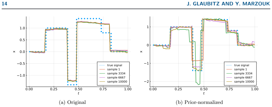
- In the impulse-image experiment, elliptical slice sampling on the normalized posterior produced more accurate reconstructions in about 15% of the runtime of a Gibbs sampler applied to the original posterior.
- MALA step sizes that were tuned for one value of the hyper-prior parameter $r$ continue to work across other values in the normalized coordinates, whereas the original posterior required step sizes an order of magnitude smaller as $r$ decreased.
- The same construction applies to any scale-mixture-of-normals prior, including Laplace and horseshoe priors, since it relies only on the conditional Gaussian structure and the hyper-prior CDF.
Reading between the lines
- If the improvement persists in higher dimensions, prior normalization could replace Gibbs sampling as the default workhorse for hierarchical Bayesian inverse problems with sparsity priors, since the normalized posterior is compatible with dimension-robust and likelihood-informed samplers.
- A natural stress test is to break the product structure: with a shared hyperparameter across coordinates, the block-diagonal map no longer exactly normalizes the prior, so the analytic derivation would need a coupled transport map and the closed form would be lost.
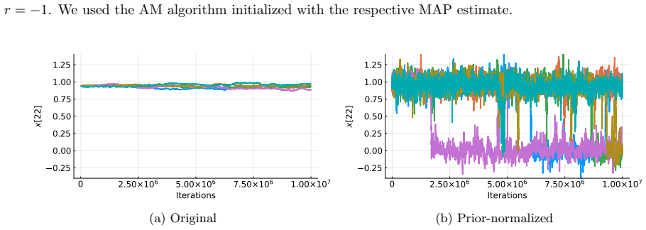
- The paper's diagnostics suggest that MPSRF and ESS can be blind to local trapping in multimodal SBL posteriors; reporting chain-level sample paths or individual posterior samples, as done here, may be the more informative check for such problems.
Editorial analysis
A structured set of objections, weighed in public.
Referee Report
Summary. The paper proposes a change of variables for sparse Bayesian learning (SBL) posteriors: a Knothe–Rosenblatt (KR) transport map that normalizes the hierarchical SBL prior to a standard normal prior. Because the SBL prior is a product over components, the high-dimensional map decouples into identical two-dimensional maps; the paper derives these maps analytically and gives a stable implementation of the inverse map in terms of generalized gamma quantile functions. The authors then compare standard MCMC algorithms (adaptive Metropolis, MALA, Gibbs, elliptical slice) on the original and prior-normalized posteriors for a toy problem, a signal deconvolution problem, a Burgers inverse problem, and an impulse-image recovery problem, and claim significant efficiency gains from prior normalization.
Significance. If the efficiency claim is supported, the paper would provide a simple, exact, and essentially parameter-free reparameterization that could improve MCMC sampling for a widely used class of hierarchical sparsity-promoting priors. The analytic derivation in Section 3 is clean and correct, the inverse map has a practical stable implementation (Appendix A), and the code is publicly available. The method does not fit any quantity to data or rely on the paper's own numerical results, so circularity is not a concern. The main open question is whether the empirical evidence actually establishes the claimed gains, and that is where the manuscript currently falls short.
major comments (3)
- [Section 4.4, Figure 17] The impulse-image experiment simultaneously changes the sampler (Gibbs for the original posterior vs. elliptical slice for the prior-normalized posterior) and the chain length (1e5 vs. 1e4 samples per chain). The reported runtime advantage and the visibly better x-mean for the prior-normalized case therefore cannot be attributed to prior normalization; they could also be due to the different sampler. To make the central claim load-bearing, please also apply the same base sampler (e.g., adaptive Metropolis or MALA) to both parameterizations in this problem, or at least report an equivalent same-sampler comparison; otherwise the abstract's claim of 'significant performance improvements' is not supported by this experiment.
- [Section 4.2, Table 3] For r = -1, the reported ESS per second is lower for the prior-normalized posterior (7.4e-1) than for the original (1.2e+0), while the MPSRF is lower for the prior-normalized posterior. The text then argues that both metrics are unreliable in multimodal settings. This is an internal tension: the only quantitative efficiency metric that favors the prior-normalized posterior is declared unreliable, and the metric that is unfavorable is also declared unreliable. The qualitative trace plots and per-chain means are suggestive but do not provide a quantitative measure of between-mode mixing. Please add a quantitative multimodal diagnostic, such as the fraction of time each chain spends in each mode, the number of transitions between the two high-density regions, or a mode-aware effective sample size, and report it for both parameterizations. Without such a diagnostic, the claim that the prior-normalized posterior is sampled more efficiently is not quantitatively established.
- [Section 4.1, Table 2] For r = 1, where the original posterior is log-concave, the original posterior yields better MPSRF and ESS than the prior-normalized posterior for both AM and MALA (e.g., MALA MPSRF 1.8e-3 vs. 2.8e-3; AM ESS/s 1.3e+5 vs. 1.0e+5). The abstract and introduction state without qualification that standard MCMC techniques sample the prior-normalized posterior more efficiently. The claim should be qualified to the non-log-concave, multimodal cases (for instance r = -1) for which the paper is arguing, and the r = 1 case should be discussed as a limitation or as evidence that prior normalization is not universally beneficial.
minor comments (6)
- [Figure 17 caption] The caption says the ES sampler generated chains 'from the original posterior' with roughly 3 minutes runtime, but the text and context indicate it sampled the prior-normalized posterior; please correct this typo.
- [Table 2 caption] The column labeled 'MPSRF' is described in the text as 'MPSRF minus one multiplied by the time'; the caption should state this explicitly so the reader knows the reported quantity is not the raw MPSRF.
- [Section 3.2, Eq. (3.2)] The product-like form relies on the assumptions that the x_i are conditionally independent given their own θ_i and that the θ_i are independent. This is exact for the SBL priors considered, but the extension to general scale mixtures of normals in Section 5 would require stating how this product structure is preserved or relaxed; otherwise the decoupling into 2D maps does not immediately apply.
- [Section 4.2] The manuscript thins the MCMC chains by keeping every 1000th sample, but it does not state whether the MPSRF and ESS values in Table 3 are computed on the thinned chains; if so, this should be reported because thinning can materially reduce the estimated ESS.
- [Figure 3] The y-axis tick labels in Figure 3 appear to be missing or unclear; adding proper axis labels or a description in the caption would improve readability.
- [Section 4.4] The runtime comparison between Gibbs and ES would be more informative if per-sample computational costs and any burn-in or adaptation period were reported, since the two samplers have very different per-iteration costs.
Circularity Check
No circular derivation; the prior-normalizing map is an explicit change of variables, and the only self-citations are background references that are not load-bearing.
full rationale
The paper's central derivation is a change of variables, not a fit or a self-referential prediction. The prior-normalizing map S is defined by the exact Knothe--Rosenblatt construction: the first component is s_theta = (Phi_0)^{-1} o P_theta (Eq. 3.6), the second is s_{x|theta} = x/sqrt(theta) (Eq. 3.5), and the inverse is t_tau = (P_theta)^{-1} o Phi_0 (Eq. 3.9) with t_{u|tau} = sqrt(t_tau(tau)) u. These formulas are explicit and derive solely from the SBL product-form prior (3.2) and standard normal CDFs; no parameter is fitted to data and no prediction is obtained from the quantity it claims to predict. The posterior identity phi_y = S#pi_y in (1.3) is the exact pushforward under the same map, so the sampling target is a genuine transformed posterior rather than a disguised input. The efficiency comparisons in Section 4 are empirical and may be confounded (for example, the Gibbs-versus-elliptical-slice comparison in Section 4.4 changes both sampler and coordinates), but confounding is a correctness or experimental-design concern, not circularity. Citations to the authors' earlier transport-map work [50, 57, 84] are background references and are not load-bearing: the KR map used here is textbook (Rosenblatt--Knothe) and is derived in the paper's own equations, with no uniqueness theorem or ansatz imported from a self-citation. The product-form assumption in (3.2) is stated explicitly and is exact for the SBL priors considered, so it is not a hidden re-import of the conclusion. On this basis, no specific circular step can be exhibited, and the appropriate finding is a low score reflecting only a minor self-citation footprint.
Assumptions & free parameters
assumptions (2)
- standard math Knothe-Rosenblatt rearrangements exist and are unique for absolutely continuous probability measures.
- domain assumption The SBL prior is a product of independent bivariate factors (x_i, θ_i), with conditionally Gaussian x_i|θ_i and generalized gamma θ_i.
Cite this review
Pith. "Pith review of Efficient sampling for sparse Bayesian learning using hierarchical prior normalization." pith.science (2026). https://pith.science/paper/YIOH4XHQ
@misc{pith2026250523753,
  author       = {Pith},
  title        = {Pith review of: Efficient sampling for sparse Bayesian learning using hierarchical prior normalization},
  year         = {2026},
  howpublished = {\url{https://pith.science/paper/YIOH4XHQ}},
  note         = {Machine review of arXiv:2505.23753}
}
read the original abstract
We introduce an approach for efficient Markov chain Monte Carlo (MCMC) sampling for challenging high-dimensional distributions in sparse Bayesian learning (SBL). The core innovation involves using hierarchical prior-normalizing transport maps (TMs), which are deterministic couplings that transform the sparsity-promoting SBL prior into a standard normal one. We analytically derive these prior-normalizing TMs by leveraging the product-like form of SBL priors and Knothe--Rosenblatt (KR) rearrangements. These transform the complex target posterior into a simpler reference distribution equipped with a standard normal prior that can be sampled more efficiently. Specifically, one can leverage the standard normal prior by using more efficient, structure-exploiting samplers. Our numerical experiments on various inverse problems -- including signal deblurring, inverting the non-linear inviscid Burgers equation, and recovering an impulse image -- demonstrate significant performance improvements for standard MCMC techniques.
Figures


Figures from the paper (14 more)




Reference graph
Works this paper leans on
-
[1]
Agapiou, J
S. Agapiou, J. M. Bardsley, O. Papaspiliopoulos, and A. M. Stuart , Analysis of the Gibbs sampler for hierarchical inverse problems, SIAM/ASA Journal on Uncertainty Quantification, 2 (2014), pp. 511–544
2014
-
[2]
Ambrosio and N
L. Ambrosio and N. Gigli , A user’s guide to optimal transport , Modelling and Optimisation of Flows on Networks, (2013), p. 1
2013
-
[3]
D. F. Andrews and C. L. Mallows , Scale mixtures of normal distributions , Journal of the Royal Statistical Society: Series B (Methodological), 36 (1974), pp. 99–102
1974
-
[4]
Andrieu and J
C. Andrieu and J. Thoms , A tutorial on adaptive MCMC , Statistics and Computing, 18 (2008), pp. 343–373
2008
-
[5]
F. Ascolani, G. O. Roberts, and G. Zanella , Scalability of Metropolis-within-Gibbs schemes for high- dimensional Bayesian models , arXiv preprint arXiv:2403.09416, (2024)
arXiv 2024
-
[6]
Y. Atchad´e and G. Fort , Limit theorems for some adaptive MCMC algorithms with subgeometric kernels , Bernoulli, 16 (2010)
work page 2010
-
[7]
Y. F. Atchad ´e, An adaptive version for the Metropolis adjusted Langevin algorithm with a truncated drift , Methodology and Computing in Applied Probability, 8 (2006), pp. 235–254
work page 2006
-
[8]
K. B. Athreya and S. N. Lahiri , Measure Theory and Probability Theory , vol. 19, Springer, 2006
work page 2006
Show all 84 references
-
[9]
S. D. Babacan, R. Molina, and A. K. Katsaggelos , Bayesian compressive sensing using Laplace priors , IEEE Transactions on Image Processing, 19 (2009), pp. 53–63. EFFICIENT SAMPLING FOR SBL USING PRIOR NORMALIZATION 23
2009
-
[10]
Baptista, Y
R. Baptista, Y. Marzouk, and O. Zahm, On the representation and learning of monotone triangular transport maps, Foundations of Computational Mathematics, (2023), pp. 1–46
2023
-
[11]
E. M. L. Beale and C. L. Mallows , Scale mixing of symmetric distributions with zero means , The Annals of Mathematical Statistics, (1959), pp. 1145–1151
1959
-
[12]
Beskos, M
A. Beskos, M. Girolami, S. Lan, P. E. F arrell, and A. M. Stuart , Geometric MCMC for infinite- dimensional inverse problems , Journal of Computational Physics, 335 (2017), pp. 327–351
2017
-
[13]
Beskos, N
A. Beskos, N. Pillai, G. Roberts, J.-M. Sanz-Serna, and A. Stuart, Optimal tuning of the hybrid Monte Carlo algorithm , Bernoulli, 19 (2013), pp. 1501–1534
2013
-
[14]
Bezanson, A
J. Bezanson, A. Edelman, S. Karpinski, and V. B. Shah , Julia: A fresh approach to numerical computing , SIAM Review, 59 (2017), pp. 65–98
2017
-
[15]
V. I. Bogachev, A. V. Kolesnikov, and K. V. Medvedev, Triangular transformations of measures, Sbornik: Mathematics, 196 (2005), p. 309
2005
-
[16]
Brooks, A
S. Brooks, A. Gelman, G. Jones, and X.-L. Meng , Handbook of Markov Chain Monte Carlo , CRC press, 2011
2011
-
[17]
S. P. Brooks and A. Gelman , General methods for monitoring convergence of iterative simulations , Journal of Computational and Graphical Statistics, 7 (1998), pp. 434–455
1998
-
[18]
Cabezas and C
A. Cabezas and C. Nemeth , Transport elliptical slice sampling , in International Conference on Artificial Intelligence and Statistics, PMLR, 2023, pp. 3664–3676
2023
-
[19]
Calvetti, M
D. Calvetti, M. Pragliola, and E. Somersalo, Sparsity promoting hybrid solvers for hierarchical Bayesian inverse problems, SIAM Journal on Scientific Computing, 42 (2020), pp. A3761–A3784
2020
-
[20]
Calvetti, M
D. Calvetti, M. Pragliola, E. Somersalo, and A. Strang , Sparse reconstructions from few noisy data: analysis of hierarchical Bayesian models with generalized gamma hyperpriors , Inverse Problems, 36 (2020), p. 025010
2020
-
[21]
Calvetti and E
D. Calvetti and E. Somersalo, A Gaussian hypermodel to recover blocky objects, Inverse Problems, 23 (2007), p. 733
2007
-
[22]
Calvetti and E
D. Calvetti and E. Somersalo , Bayesian Scientific Computing , vol. 215, Springer Nature, 2023
2023
-
[23]
Calvetti and E
D. Calvetti and E. Somersalo , Computationally efficient sampling methods for sparsity promoting hierar- chical Bayesian models , SIAM/ASA Journal on Uncertainty Quantification, 12 (2024), pp. 524–548
2024
-
[24]
Calvetti, E
D. Calvetti, E. Somersalo, and A. Strang , Hierachical Bayesian models and sparsity: ℓ2-magic, Inverse Problems, 35 (2019), p. 035003
2019
-
[25]
C. M. Carvalho, N. G. Polson, and J. G. Scott, Handling sparsity via the horseshoe, in Artificial Intelligence and Statistics, PMLR, 2009, pp. 73–80
2009
-
[26]
N. K. Chada, M. A. Iglesias, L. Roininen, and A. M. Stuart , Parameterizations for ensemble Kalman inversion, Inverse Problems, 34 (2018), p. 055009
2018
-
[27]
V. Chen, M. M. Dunlop, O. Papaspiliopoulos, and A. M. Stuart , Robust MCMC sampling with non- Gaussian and hierarchical priors in high dimensions , arXiv preprint arXiv:1803.03344, 3 (2018)
2018 arXiv
-
[28]
Churchill and A
V. Churchill and A. Gelb , Sampling-based spotlight SAR image reconstruction from phase history data for speckle reduction and uncertainty quantification , SIAM/ASA Journal on Uncertainty Quantification, 10 (2022), pp. 1225–1249
2022
-
[29]
Cotter, G
S. Cotter, G. Roberts, A. Stuart, and D. White, MCMC methods for functions: Modifying old algorithms to make them faster , Statistical Science, 28 (2013), pp. 424–446
2013
-
[30]
T. Cui, X. T. Tong, and O. Zahm , Prior normalization for certified likelihood-informed subspace detection of Bayesian inverse problems , Inverse Problems, 38 (2022), p. 124002
2022
-
[31]
https://dlmf.nist.gov/, Release 1.2.0 of 2024-03-15
NIST Digital Library of Mathematical Functions . https://dlmf.nist.gov/, Release 1.2.0 of 2024-03-15. F. W. J. Olver, A. B. Olde Daalhuis, D. W. Lozier, B. I. Schneider, R. F. Boisvert, C. W. Clark, B. R. Miller, B. V. Saunders, H. S. Cohl, and M. A. McClain, eds
2024
-
[32]
Dong and M
Y. Dong and M. Pragliola, Inducing sparsity via the horseshoe prior in imaging problems , Inverse Problems, 39 (2023), p. 074001
2023
-
[33]
M. M. Dunlop, T. Helin, and A. M. Stuart , Hyperparameter estimation in Bayesian MAP estimation: parameterizations and consistency, The SMAI Journal of Computational Mathematics, 6 (2020), pp. 69–100
2020
-
[34]
M. A. Figueiredo, J. M. Bioucas-Dias, and R. D. Nowak , Majorization–minimization algorithms for wavelet-based image restoration, IEEE Transactions on Image Processing, 16 (2007), pp. 2980–2991
2007
-
[35]
Fleischer , Transformations for accelerating MCMC simulations with broken ergodicity , in 2007 Winter Simulation Conference, IEEE, 2007, pp
M. Fleischer , Transformations for accelerating MCMC simulations with broken ergodicity , in 2007 Winter Simulation Conference, IEEE, 2007, pp. 658–666
2007
-
[36]
Flock, Y
R. Flock, Y. Dong, F. Uribe, and O. Zahm , Continuous Gaussian mixture solution for linear Bayesian 24 J. GLAUBITZ AND Y. MARZOUK inversion with application to Laplace priors , Inverse Problems, (2024)
2024
-
[37]
Gelman, J
A. Gelman, J. B. Carlin, H. S. Stern, and D. B. Rubin, Bayesian Data Analysis, Chapman and Hall/CRC, 2003
2003
-
[38]
Gelman and D
A. Gelman and D. B. Rubin , Inference from iterative simulation using multiple sequences , Statistical Science, 7 (1992), pp. 457–472
1992
-
[39]
Glaubitz and A
J. Glaubitz and A. Gelb , Leveraging joint sparsity in hierarchical Bayesian learning , SIAM/ASA Journal on Uncertainty Quantification, 12 (2024), pp. 442–472
2024
-
[40]
Glaubitz, A
J. Glaubitz, A. Gelb, and G. Song , Generalized sparse Bayesian learning and application to image recon- struction, SIAM/ASA Journal on Uncertainty Quantification, 11 (2023), pp. 262–284
2023
-
[41]
Gom `es, C
O. Gom `es, C. Combes, and A. Dussauchoy , Parameter estimation of the generalized gamma distribution , Mathematics and Computers in Simulation, 79 (2008), pp. 955–963
2008
-
[42]
Haario, E
H. Haario, E. Saksman, and J. Tamminen , An adaptive Metropolis algorithm , Bernoulli, 7 (2001), pp. 223– 242
2001
-
[43]
Kaipio and E
J. Kaipio and E. Somersalo , Statistical inverse problems: discretization, model reduction and inverse crimes , Journal of Computational and Applied Mathematics, 198 (2007), pp. 493–504
2007
-
[44]
Knothe, Contributions to the theory of convex bodies
H. Knothe, Contributions to the theory of convex bodies. , Michigan Mathematical Journal, 4 (1957), pp. 39–52
1957
-
[45]
Lindbloom, J
J. Lindbloom, J. Glaubitz, and A. Gelb , Efficient sparsity-promoting MAP estimation for Bayesian linear inverse problems, Inverse Problems, 41 (2025), p. 025001
2025
-
[46]
Lindbloom, M
J. Lindbloom, M. Pasha, J. Glaubitz, and Y. Marzouk , Priorconditioned sparsity-promoting projection methods for deterministic and Bayesian linear inverse problems , arXiv preprint arXiv:2505.01827, (2025)
2025 arXiv
-
[47]
J. S. Liu , Monte Carlo Strategies in Scientific Computing , Springer Science & Business Media, 2013
2013
-
[48]
Markkanen, L
M. Markkanen, L. Roininen, J. M. Huttunen, and S. Lasanen, Cauchy difference priors for edge-preserving Bayesian inversion , Journal of Inverse and Ill-Posed Problems, 27 (2019), pp. 225–240
2019
-
[49]
Marshall and G
T. Marshall and G. Roberts , An adaptive approach to Langevin MCMC , Statistics and Computing, 22 (2012), pp. 1041–1057
2012
-
[50]
Marzouk, T
Y. Marzouk, T. Moselhy, M. Parno, and A. Spantini , Sampling via measure transport: An introduction , Handbook of Uncertainty Quantification, 1 (2016), p. 2
2016
-
[51]
Murray, R
I. Murray, R. Adams, and D. MacKay , Elliptical slice sampling , in Proceedings of the 13th International Conference on Artificial Intelligence and Statistics, 2010, pp. 541–548
2010
-
[52]
Nishihara, I
R. Nishihara, I. Murray, and R. P. Adams , Parallel MCMC with generalized elliptical slice sampling , The Journal of Machine Learning Research, 15 (2014), pp. 2087–2112
2014
-
[53]
Nocedal and S
J. Nocedal and S. J. Wright , Numerical Optimization, Springer, 2006
2006
-
[54]
Papaspiliopoulos, G
O. Papaspiliopoulos, G. O. Roberts, and M. Sk¨old, Non-centered parameterisations for hierarchical models and data augmentation , Bayesian Statistics, 7 (2003), pp. 307–326
2003
-
[55]
Papaspiliopoulos, G
O. Papaspiliopoulos, G. O. Roberts, and M. Sk ¨old, A general framework for the parametrization of hier- archical models, Statistical Science, (2007), pp. 59–73
2007
-
[56]
Park and G
T. Park and G. Casella , The Bayesian Lasso , Journal of the American Statistical Association, 103 (2008), pp. 681–686
2008
-
[57]
M. D. Parno and Y. M. Marzouk, Transport map accelerated Markov chain Monte Carlo, SIAM/ASA Journal on Uncertainty Quantification, 6 (2018), pp. 645–682
2018
-
[58]
F. J. Pinski, G. Simpson, A. M. Stuart, and H. Weber , Algorithms for Kullback–Leibler approximation of probability measures in infinite dimensions , SIAM Journal on Scientific Computing, 37 (2015), pp. A2733– A2757
2015
-
[59]
Rackauckas and Q
C. Rackauckas and Q. Nie , DifferentialEquations.jl – A performant and feature-rich ecosystem for solving differential equations in Julia , Journal of Open Research Software, 5 (2017), p. 15
2017
-
[60]
Ranocha, M
H. Ranocha, M. Schlottke-Lakemper, A. R. Winters, E. F aulhaber, J. Chan, and G. J. Gassner , Adaptive numerical simulations with Trixi.jl: A case study of Julia for scientific computing , Proceedings of the JuliaCon Conferences, 1 (2022), p. 77
2022
-
[61]
Ranocha, A
H. Ranocha, A. R. Winters, M. Schlottke-Lakemper, P. ¨Offner, J. Glaubitz, and G. J. Gassner, On the robustness of high-order upwind summation-by-parts methods for nonlinear conservation laws , Journal of Computational Physics, 520 (2025), p. 113471
2025
-
[62]
Rezende and S
D. Rezende and S. Mohamed , Variational inference with normalizing flows , in International Conference on Machine Learning, PMLR, 2015, pp. 1530–1538
2015
-
[63]
Robert and G
C. Robert and G. Casella , Monte Carlo Statistical Methods , Springer Science & Business Media, 2013
2013
-
[64]
G. O. Roberts and J. S. Rosenthal , Optimal scaling of discrete approximations to Langevin diffusions , EFFICIENT SAMPLING FOR SBL USING PRIOR NORMALIZATION 25 Journal of the Royal Statistical Society: Series B (Statistical Methodology), 60 (1998), pp. 255–268
1998
-
[65]
Rosenblatt, Remarks on a multivariate transformation , The Annals of Mathematical Statistics, 23 (1952), pp
M. Rosenblatt, Remarks on a multivariate transformation , The Annals of Mathematical Statistics, 23 (1952), pp. 470–472
1952
-
[66]
Santambrogio, Optimal Transport for Applied Mathematicians , Springer, 2015
F. Santambrogio, Optimal Transport for Applied Mathematicians , Springer, 2015
2015
-
[67]
Sanz-Alonso and O
D. Sanz-Alonso and O. Al-Ghattas, A first course in Monte Carlo methods, arXiv preprint arXiv:2405.16359, (2024)
2024 arXiv
-
[68]
Sanz-Alonso and N
D. Sanz-Alonso and N. W aniorek , Hierarchical Bayesian inverse problems: A high-dimensional statistics viewpoint, arXiv preprint arXiv:2401.03074, (2024)
2024 arXiv
-
[69]
Z. Si, Y. Liu, and A. Strang , Path-following methods for maximum a posteriori estimators in Bayesian hierarchical models: How estimates depend on hyperparameters , SIAM Journal on Optimization, 34 (2024), pp. 2201–2230
2024
-
[70]
A. M. Stuart, Inverse problems: a Bayesian perspective , Acta Numerica, 19 (2010), pp. 451–559
2010
-
[71]
Suuronen, N
J. Suuronen, N. K. Chada, and L. Roininen , Cauchy Markov random field priors for Bayesian inversion , Statistics and Computing, 32 (2022), p. 33
2022
-
[72]
X. Tan, J. Li, and P. Stoica, Efficient sparse bayesian learning via Gibbs sampling, in 2010 IEEE International Conference on Acoustics, Speech and Signal Processing, IEEE, 2010, pp. 3634–3637
2010
-
[73]
M. E. Tipping , Sparse Bayesian learning and the relevance vector machine , Journal of Machine Learning Re- search, 1 (2001), pp. 211–244
2001
-
[74]
Uribe, J
F. Uribe, J. M. Bardsley, Y. Dong, P. C. Hansen, and N. A. Riis , A hybrid Gibbs sampler for edge- preserving tomographic reconstruction with uncertain view angles, SIAM/ASA Journal on Uncertainty Quan- tification, 10 (2022), pp. 1293–1320
2022
-
[75]
Uribe, Y
F. Uribe, Y. Dong, and P. C. Hansen, Horseshoe priors for edge-preserving linear Bayesian inversion , SIAM Journal on Scientific Computing, 45 (2023), pp. B337–B365
2023
-
[76]
Vehtari, A
A. Vehtari, A. Gelman, D. Simpson, B. Carpenter, and P.-C. B ¨urkner, Rank-normalization, folding, and localization: An improved ˆR for assessing convergence of MCMC (with discussion) , Bayesian Analysis, 16 (2021), pp. 667–718
2021
-
[77]
Villani, Optimal Transport: Old and New , vol
C. Villani, Optimal Transport: Old and New , vol. 338, Springer, 2009
2009
-
[78]
W ang, J
Z. W ang, J. M. Bardsley, A. Solonen, T. Cui, and Y. M. Marzouk , Bayesian inverse problems with ℓ1 priors: a randomize-then-optimize approach , SIAM Journal on Scientific Computing, 39 (2017), pp. S140– S166
2017
-
[79]
West, On scale mixtures of normal distributions , Biometrika, 74 (1987), pp
M. West, On scale mixtures of normal distributions , Biometrika, 74 (1987), pp. 646–648
1987
-
[80]
D. P. Wipf and B. D. Rao , Sparse Bayesian learning for basis selection , IEEE Transactions on Signal Pro- cessing, 52 (2004), pp. 2153–2164
2004
-
[81]
Wolff and A
U. Wolff and A. Collaboration , Monte Carlo errors with less errors , Computer Physics Communications, 156 (2004), pp. 143–153
2004
-
[82]
Xiao and J
Y. Xiao and J. Glaubitz , Sequential image recovery using joint hierarchical Bayesian learning , Journal of Scientific Computing, 96 (2023), p. 4
2023
-
[83]
J. Yang, G. O. Roberts, and J. S. Rosenthal , Optimal scaling of random-walk Metropolis algorithms on general target distributions , Stochastic Processes and their Applications, 130 (2020), pp. 6094–6132
2020
-
[84]
O. Zahm, T. Cui, K. Law, A. Spantini, and Y. Marzouk , Certified dimension reduction in nonlinear Bayesian inverse problems , Mathematics of Computation, 91 (2022), pp. 1789–1835
2022
Reviewed August 7, 2026 · model on record in the stance chip above.
Discussion (0). Sign in to comment.