REVIEW 2 major objections 4 minor 2 cited by
Paired comparison models with strength-dependent ties and order effects
T0 review · 2 major / 4 minor · reviewed 2026-08-07 · deepseek-v4-flash
Pith's one-line read The paper proposes that in chess-like paired comparisons, both draw probability and the white-pieces order advantage grow with the average strength of the two players, and that a model encoding this beats constant-effect alternatives on…
desk verdict A solid extension of David's paired comparison model with a well-supported strength-dependent draw effect, but the strength-dependent order effect is not backed by the paper's own posterior interval. read the letter →
The pith
A machine-rendered reading of the paper's core claim, the machinery that carries it, and where it could break.
The reading
What carries the argument
The machine is equation (6), a three-outcome multinomial logit. For a match between $i$ and $j$, the win and loss numerators carry the order effect $\alpha_0+\alpha_1(\theta_i+\theta_j)/2$ inside terms of the form $\exp(\theta_i \pm x_{ij}(\alpha_0+\alpha_1(\theta_i+\theta_j)/2)/4)$, and the draw numerator is $\exp(\beta_0+(1+\beta_1)(\theta_i+\theta_j)/2)$, all normalized by their sum $D_{ij}$. The object doing the work is the pair-average strength $(\theta_i+\theta_j)/2$, which enters both the tie log-odds and the order effect; setting $\alpha_1=\beta_1=0$ recovers the constant-parameter model, making that model a nested special case and giving the comparison a direct likelihood-based interpretation.
What would settle it
Re-estimate the model on a large chess dataset, or on another tie-heavy sport, with smooth splines replacing the linear average-strength terms and compare DIC; if the spline version fits better, or if the posterior interval for $\alpha_1$ is not positive, then the strength-dependent order-effect claim is unsupported even though the draw side may survive.
Extended reading notes
Core claim
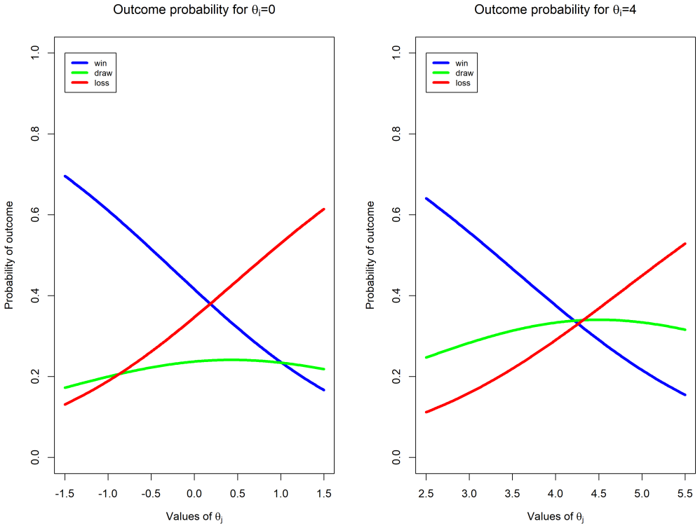
The central claim is that strength-dependence belongs in the model itself, not in the residual. Specifically, the paper's equation (6) replaces the fixed tie log-odds with $\exp(\beta_0+(1+\beta_1)(\theta_i+\theta_j)/2)$, so that $\beta_1 > 0$ means stronger pairs draw more often, and replaces the fixed order effect with $\alpha_0+\alpha_1(\theta_i+\theta_j)/2$, so that $\alpha_1>0$ means the white advantage grows with average strength. The full model has $\beta_1=0.120$ with 95% interval (0.103, 0.138) and $\alpha_1=0.037$ with 95% interval (0.000, 0.074), and beats all six variants tried on the US Open data, including the constant-parameter model, by a DIC margin of more than 800. The win-versus-loss odds remain independent of the tie parameters, so the extension preserves the standard property of the tie model while letting draw and order effects move with skill.
Load-bearing premise
The load-bearing premise is that the order effect grows linearly with average player strength, a premise that is fragile because the posterior interval for $\alpha_1$ includes zero, so if the true coefficient is not positive or the growth is not linear the order-effect half of the central claim collapses even though the model still fits better through the draw parameter $\beta_1$.
Editorial extensions
If this is right
- If the central claim is correct, the constant tie and order-effect model that has been standard for paired comparisons is misspecified for chess-like data, with a DIC gap of roughly 835 points.
- The model predicts that two strong evenly matched players draw about 49% of the time, versus about 24% for two average evenly matched players, a pattern testable in any large chess database.
- The white advantage in win-to-loss odds rises from about 1.2 for average pairs to about 1.244 for strong pairs, so rankings that ignore this will slightly overstate weaker players' results when they play white.
- The same three-outcome structure can be fitted with standard Bayesian software to any paired-comparison sport with draws and home advantage, such as soccer or hockey.
- Because the model nests the constant-parameter model, existing likelihood-ratio and DIC comparisons can be used to test for strength dependence in new datasets without changing the estimation setup.
Reading between the lines
- The draw-side of the claim is well supported; the order-effect side is fragile because $\alpha_1$'s posterior interval includes zero, so a conservative reading would treat only the strength-dependent tie rate as established.
- In soccer-like settings where home advantage and draws both matter, the same structure transfers directly: one would expect draw rates to rise when two top teams meet, and a nonlinear version could be tested with splines.
- Because player-years are treated as independent, the strength-dependent effects could be confounded with rating inflation or age trends; a longitudinal version would separate these dynamics.
- If the true tie effect is nonlinear, the linear term $\beta_1$ may still win by DIC while mispredicting at very high strengths; fitting a monotone spline version would be a sharper test of the mechanism.
Editorial analysis
A structured set of objections, weighed in public.
Referee Report
Summary. The paper proposes an extension of David (1988) paired comparison models in which both the tie probability and the order effect depend on the average strength of the two players (Eq. (6)). The model is motivated by GAM analyses on FIDE data, fitted to 24,888 US Chess Open games under six model variants and two priors, and compared by DIC. The strength-dependent tie parameter is estimated as β1 = 0.120 with interval (0.103, 0.138), supporting the first phenomenon. The strength-dependent order-effect parameter is estimated as α1 = 0.037 with interval (0.000, 0.074), which includes zero, and the corresponding GAM is explicitly described as less conclusive.
Significance. If taken as a modeling proposal, the paper contributes a clean, interpretable extension of a standard paired comparison framework, and the first empirical phenomenon (stronger pairs draw more often) is well supported by a tight posterior interval. The design is also a strength: the exploratory GAM analysis uses FIDE data while the confirmatory model fitting uses US Open data, reducing circularity concerns. However, the second headline phenomenon is not established by the reported posterior, and the in-sample DIC comparison does not by itself justify the language of predictive performance. The result is a sound model with one strong empirical finding and one suggestive but unconfirmed finding.
major comments (2)
- [Section 3, Eq. (6); Section 4, Table 4] The strength-dependent order effect is not empirically established. The posterior mean α1 = 0.037 has a 95% central interval (0.000, 0.074), so the data are consistent with α1 = 0; the GAM motivating this effect (Figure 2) is itself described in Section 2 as 'less conclusive'. The statement in Section 4 that 'The value of α1 being inferred to be positive indicates that the advantage to playing white increases slightly as a function of the players' strengths' is therefore an overstatement. Since the abstract and introduction present strength-dependent order effects as one of the two phenomena the model addresses, this is load-bearing for the central claim. The paper should either soften the claim to a model assumption with suggestive support or provide additional evidence that discriminates α1 > 0, such as out-of-sample prediction, prior sensitivity analysis, or a smoother estimate of the average-strength effect.
- [Section 4, Table 3; Section 5] The claim of 'clear improvements in predictive performance' is based on DIC values computed on the same data used for fitting. DIC is an in-sample approximation to out-of-sample predictive error, not a validation exercise, and the DIC ordering across nested models is not obviously stable: under the informative prior, Model 2 (no color effect) has lower DIC than Model 3 (constant color effect), despite the posterior for α0 being positive. To support the predictive language, the paper should add out-of-sample or cross-validated predictive comparisons, or at minimum change the wording to 'better fit' and discuss the instability.
minor comments (4)
- [Section 3, Eq. (8)] The notation in Eq. (8) uses K for the number of games and then refers to θ = (θ1, ..., θK), although θ has n player components; use n for the number of players to avoid confusion.
- [Section 4, prior specification] The invariance claim 'our model is invariant to additive shifts to the strength parameters' is correct only as a joint transformation: under θ_i → θ_i + c, invariance requires α0 → α0 − α1 c and β0 → β0 − β1 c. Stating this explicitly would clarify the role of the rating-scale origin.
- [Table 3] The DIC comparison shows that Model 2 (no color effect) outperforms Model 3 (constant color effect) under the informative prior, which is surprising in light of the posterior for α0; a sentence of explanation would help readers interpret the model-selection results.
- [Section 2, GAM details] For the GAM analyses, reporting the effective degrees of freedom and the basis used for the smoothing splines would improve reproducibility; the current text only says 'cubic smoothing spline'.
Circularity Check
No significant circularity: the central parameters are estimated from data, not defined into existence.
full rationale
Walking the claimed derivation chain, the paper proposes an explicit parametric extension of David's model in equation (6), fits it by MCMC to US Chess Open game outcomes, and compares DIC values across special cases (Table 3) and posterior intervals (Table 4). The two substantive claims, that stronger pairs draw more often and that order effects grow with strength, are empirical inferences from the free parameters beta_1 and alpha_1, not consequences of the model definition. beta_1 is identified by the likelihood, and its posterior interval (0.103, 0.138) is data-driven; alpha_1's interval includes 0, which is a statistical-evidence weakness, not circularity. The exploratory GAM on FIDE data (Figures 1 and 2) is independent motivation, and the confirmatory fit on a separate US Open dataset is an appropriate validation design rather than a circular reuse of the same fitted values. The only self-citation, Glickman and Jones (2024), supports the standard Elo-to-Bradley-Terry rating conversion used to set prior means; it is not load-bearing for the central inference, and the conversion is a conventional external result. The model's lack of invariance to additive shifts when alpha_1 and beta_1 are nonzero is a modeling and identifiability concern, but it is not a case of a fitted input being renamed as a prediction or of an equation reducing to its own input. No step in the paper exhibits the required pattern of circularity.
Assumptions & free parameters
free parameters (9)
- α0 =
0.363 (0.289, 0.434)
- α1 =
0.037 (0.000, 0.074)
- β0 =
-0.471 (-0.505, -0.437)
- β1 =
0.120 (0.103, 0.138)
- σ =
0.645 (0.604, 0.687)
- μ_miss =
-3.399 (-4.110, -2.703)
- σ_miss =
2.636 (2.085, 3.310)
- Strength prior hyperparameters
- Non-strength parameter prior variances
assumptions (4)
- domain assumption Luce's choice axiom / IIA: outcome probabilities are proportional to exponentials of linear terms, with the draw treated as a third multinomial category.
- domain assumption US Chess and FIDE ratings are linear transformations of Bradley-Terry log-strength parameters, so μ_i=(R_i-1500)/(400/log10) is the prior mean for θ_i.
- domain assumption Independent normal priors on θ, α0, α1, β0, β1 and diffuse inverse-Gamma priors on variances yield a proper posterior and converged MCMC.
- domain assumption Players who appear in multiple US Opens can be treated as distinct players, so repeated participation does not create within-player correlation.
Cite this review
Pith. "Pith review of Paired comparison models with strength-dependent ties and order effects." pith.science (2026). https://pith.science/paper/KQYPEZNP
@misc{pith2026250524783,
  author       = {Pith},
  title        = {Pith review of: Paired comparison models with strength-dependent ties and order effects},
  year         = {2026},
  howpublished = {\url{https://pith.science/paper/KQYPEZNP}},
  note         = {Machine review of arXiv:2505.24783}
}
read the original abstract
Paired comparison models, such as the Bradley-Terry (1952) model and its variants, are commonly used to measure competitor strength in games and sports. Extensions have been proposed to account for order effects (e.g., home-field advantage) as well as the possibility of a tie as a separate outcome, but such models are rarely adopted in practice due to poor fit with actual data. We propose a novel paired comparison model that accounts not only for ties and order effects, but recognizes two phenomena that are not addressed with commonly used models. First, the probability of a tie may be greater for stronger pairs of competitors. Second, order effects may be more pronounced for stronger competitors. This model is motivated in the context of tournament chess game outcomes. The models are demonstrated on the results of US Chess Open game outcomes from 2006 to 2019, large tournaments consisting of players of wide-ranging strengths.
Figures


Figures from the paper (2 more)

Forward citations
Cited by 2 Pith papers
-
Tied Pools and Drawn Games
Draws should count as half-wins when estimating chess strength, with draw frequency estimated afterward; this justifies Glickman's rule and is applied to an 1821 chess pool.
-
Rating competitors in games with strength-dependent tie probabilities
A Bayesian rating system that models draw probability as increasing with player strength, with fast one-step posterior updates, is developed and deployed on ICCF chess data.
Reference graph
Works this paper leans on
-
[1]
Baker, R. D. & Scarf, P. A. (2020), ‘Modifying Bradley–Terry and other ranking models to allow ties’,IMA Journal of Management Mathematics32(4), 451–463. Bezdek, J. & Hathaway, R. (2002), Some notes on alternating optimization,inN. R. Pal & M. Sugeno, eds, ‘Advances in Soft Computing —AFSS 2002’, Springer, Berlin, Heidelberg, pp. 288–300. 22 Bradley, R. A...
work page 2020
-
[9]
Plummer, M. (2003), JAGS: A program for analysis of Bayesian graphical models using Gibbs sampling,in‘Proceedings of the 3rd International Workshop on Distributed Statistical Computing (DSC 2003). March’, pp. 20–22. 23 Spiegelhalter, D. J., Best, N. G., Carlin, B. P. & Van Der Linde, A. (2002), ‘Bayesian measures of model complexity and fit’,Journal of th...
work page 2003
-
[333]
Hastie, T. & Tibshirani, R. (1986), ‘Generalized additive models’,Statistical science 1(3), 297–310. Ma, S. (2015), ‘Alternating proximal gradient method for convex minimization’,Journal of Scientific Computing68, 546 –
work page 1986
-
[572]
(1951), ‘Remarks on the method of paired comparisons: I
Mosteller, F. (1951), ‘Remarks on the method of paired comparisons: I. The least squares so- lution assuming equal standard deviations and equal correlations’,Psychometrika16(1), 3–
work page 1951
Reviewed August 7, 2026 · model on record in the stance chip above.
Discussion (0). Sign in to comment.