Girth and Laplacian eigenvalue distribution

Bo Zhou; Leyou Xu

REVIEW 2 major objections 3 minor 34 references

Girth and Laplacian eigenvalue distribution

T0 review · 2 major / 3 minor · reviewed 2026-08-07 · deepseek-v4-flash

Challenge this review Re-run · record.json Download PDF Read on arXiv ↗

Pith's one-line read This paper proves that in any connected graph of order n and girth at least 4, at most n−g Laplacian eigenvalues lie in the interval [n−g−k+4, n] for every k up to min{g−1, n−g}, and it determines the extremal graphs for k=1 and k=2.

desk verdict A useful sharp bound with a repairable gap in the k≥3 case; worth refereeing after the authors fix the S3=∅ subcase and show the claimed finite eigenvalue checks. read the letter →

arxiv 2506.00921 v1 pith:KEH5A75J submitted 2025-06-01 math.CO

Leyou Xu , Bo Zhou This is my paper

classification math.CO MSC 05C5015A1805C38

keywords Laplacianeigenvaluedistributiongirthcycleextremalgraphtheoryspectralspectrummatrixinterlacingcompletebipartite

verification ladder T0 review T1 audit T2 compute T3 formal

The pith

A machine-rendered reading of the paper's core claim, the machinery that carries it, and where it could break.

The reading

The paper establishes a precise link between a graph's girth—the length of its shortest cycle—and the distribution of its largest Laplacian eigenvalues. For a connected graph $G$ of order $n$ and girth $g\ge 4$, it proves that for every $k=1,\ldots,\min\{g-1,n-g\}$, the interval $[n-g-k+4,n]$ contains at most $n-g$ Laplacian eigenvalues, counting multiplicity. The bound is attained for $k=1$ and $k=2$ only by explicitly listed graphs, and the paper determines those graphs completely. For girth $3$, it classifies all connected graphs for which the relevant top intervals contain $n-1$, $n-2$, or $n-3$ eigenvalues. These results matter because they turn a purely combinatorial parameter—the shortest cycle—into a quantitative control on the spectral distribution, a connection previously available only for the narrowest window.

What carries the argument

The central object is the subgraph $H=G[V(C)\cup S]$ formed by a shortest cycle $C$ of length $g$ together with a set $S$ of $k$ vertices outside it. The load-bearing inequality is $\mu_{k+1}(H)<4$, which the proof establishes for every allowed configuration; interlacing (Lemma 5) and Weyl's inequality (Lemma 4) then give $\mu_{n-g+1}(G)\le \mu_{k+1}(H)+n-g-k$, so the eigenvalue-count bound follows. The verification of $\mu_{k+1}(H)<4$ is carried out by a case analysis on how the outside vertices attach to the cycle and to one another, using the known spectra of paths, cycles, and complete bipartite graphs, the edge-deletion interlacing principle, and several direct numerical computations for small exceptional graphs.

What would settle it

Compute the full Laplacian spectra of the small graphs $R_1,R_2,R_3,Q_1,Q_2,Q_3,Q_4,F_0,F_1,F_2$ by exact arithmetic and check the asserted inequalities (for example $\mu_3(R_i)<5$, $\mu_5(Q_1)=2.555$, $\mu_5(Q_2)=2$, $\mu_5(Q_4)=2.746$); if any is false, or if an exhaustive computer search over connected graphs of order at most 10 finds a graph of girth $\ge 4$ with more than $n-g$ eigenvalues in $[n-g-k+4,n]$ for some allowed $k$, the theorem collapses.

Watch

Extended reading notes

Core claim

The central discovery is Theorem 2: if $G$ is a connected graph with $n$ vertices and girth $g\ge 4$, then for each $k=1,\ldots,\min\{g-1,n-g\}$, the number of Laplacian eigenvalues of $G$ in $[n-g-k+4,n]$ is at most $n-g$. The proof achieves this by selecting a shortest cycle $C$ of length $g$ and $k$ vertices $S$ outside it, forming the induced subgraph $H$ on $V(C)\cup S$, and showing that the $(k+1)$-th Laplacian eigenvalue of $H$ is below $4$; interlacing and a Weyl-type inequality then transfer this small-subgraph fact into the bound for $G$. Equality for $k=1$ forces $g=n-1$ with $G\cong K_{2,3}$ or $U_n$, while equality for $k=2$ forces $G$ to be one of $K_{2,4}$, the three graphs $K^*_{2,3}, K^{**}_{2,3}, K^{***}_{2,3}$, or a graph $Y_{n,i}$ in which two extra vertices attach to a cycle $C_{n-2}$ at specified distances. For girth $3$, Theorem 3 classifies the graphs with $n-1$, $n-2$, or $n-3$ Laplacian eigenvalues in the top interval, expressed in terms of complete graphs with certain edges deleted and joins of complete graphs with independent sets.

Load-bearing premise

The bound for $k\ge 3$ rests on the assertion that the $(k+1)$-th largest Laplacian eigenvalue of the subgraph built from a shortest cycle plus $k$ outside vertices is always below $4$; that assertion is verified by a case analysis that relies on unshown numerical checks and on the completeness of the listed attachment patterns.

Editorial extensions

If this is right

If $G$ is connected with girth $g\ge 4$, then for each $k\le \min\{g-1,n-g\}$ at most $n-g$ Laplacian eigenvalues lie in $[n-g-k+4,n]$; in particular, for $k=1$ the interval $[n-g+3,n]$ holds at most $n-g$ eigenvalues.
Equality for $k=1$ occurs exactly when $g=n-1$, and the only such graphs are $K_{2,3}$ and $U_n$; equality for $k=2$ occurs exactly for the explicit list in Theorem 4, including $K_{2,4}$, the three variants of $K_{2,3}$, and the family $Y_{n,i}$.
For girth $3$, a connected graph has $n-1$ or $n-2$ Laplacian eigenvalues equal to $n$ only when it is $K_n$ or $K_n$ with one edge removed, respectively; the $n-3$ case is exactly the three joins $K_{n-3}\vee 3K_1$, $K_{n-3}\vee (K_1\cup K_2)$, and $K_{n-4}\vee 2K_2$.
For girth $3$ and the interval $[n-1,n]$, the $n-1$ and $n-2$ cases occur only for $K_n$ and for complete graphs with all edges at one vertex deleted, respectively, with the $n-3$ case classified into the families $H(n)$, $H(n,a)$, and three edge-deleted complete graph families (a), (b), (c).
Because at most $n-g$ eigenvalues lie in the top window, at least $g$ Laplacian eigenvalues must lie below $n-g-k+4$, so the theorem gives a lower bound on how many eigenvalues are 'small' in terms of girth alone.

Reading between the lines

Editorial extensions of the paper, not claims the author makes directly.

It is plausible the same reduction to a small subgraph $H$ could be repeated with other cycle parameters—odd girth, circumference, or cyclomatic number—to produce analogous top-window bounds for the Laplacian spectrum.
The equality classification for $k=2$ is very rigid; for $k\ge 3$ the paper only gives examples showing sharpness, so a natural next step would be a computational search over small graphs to guess the full equality families.
The 'direct calculation' spectral values (such as $\mu_5(Q_1)=2.555$, $\mu_5(Q_2)=2$, $\mu_5(Q_4)=2.746$) are stated without derivation; an independent exact computation of these small graphs would be a quick check on the proof's finite verification step, and if any value differs the bound might still survive through a different numerical route.
The theorem implies that graphs with large girth have a relatively small number of large Laplacian eigenvalues; since the number of vertices outside a shortest cycle is $n-g$, the bound matches intuition that each vertex outside the cycle contributes at most one eigenvalue to the top window.

Share X Bluesky LinkedIn Reddit HN

Editorial analysis

A structured set of objections, weighed in public.

Desk editor's note, referee report, and a circularity audit.

Desk Editor's Note

read the letter

Here's my take on arXiv:2506.00921. The genuinely new content is the girth-4+ bound for all k (Theorem 2 for k≥3) and the k=2 equality classification; the prior work [33] only handled k=1. The proof strategy is sound in outline: choose a shortest cycle, take k outside vertices, use interlacing to reduce to showing the induced subgraph H has µ_{k+1}(H)<4, then split into cases. The case analysis is laborious but mostly standard.

The stress-test note is correct, and it lands on a real gap. In Section 4, Case 1.1, when S1=∅ and S3=∅, all k vertices of S are pendant leaves attached to the cycle. The asserted bound |E(S)| ≤ |S3|−1 is false there: |E(S)|=0 but |S3|−1=−1. Consequently |E0| can equal k, and the interlacing gives only µ_{k+1}(H) ≤ µ_1(C_g)=4, not the strict <4 the proof needs. This is not a missing numerical check; it is the only argument for that exhaustive subcase. I suspect the bound is still true—one can delete k−1 of the cycle–leaf edges and bound µ_2 of a cycle with one pendant leaf—but the written proof does not do that.

There are also quite a few eigenvalue bounds asserted as 'direct calculation' with no spectra shown (e.g., µ_5(Q1)=2.555, µ_5(Q2)=2, µ_5(Q4)=2.746, and the µ_2 values for R2,R3). Those are finite checks and probably fine, but they are load-bearing for the equality classifications, so a referee should ask for them to be displayed or verified.

The girth-3 section leans heavily on the authors' own previous classification theorems [29,30]; the genuinely new part is the n−3 case, which is not derived from first principles but is a mixture of restatement and new cases. The paper is transparent about this, and the abstract's phrasing is a bit overbroad but not dishonest.

Overall: the main bound is likely true and is a real extension of the k=1 result. The proof has a repairable gap and some opaque finite computations. It deserves peer review and a serious referee who will push for the missing details. I would not cite it until the gap is closed.

Referee Report

2 major / 3 minor

Summary. The paper studies the number of Laplacian eigenvalues of a connected graph in a top interval whose left endpoint depends on the order n, the girth g, and an integer k. For girth at least 4, Theorem 2 claims that for every k up to min{g-1,n-g}, at most n-g eigenvalues lie in [n-g-k+4,n], with equality classifications for k=1 and k=2. Theorem 3 gives analogous classifications for graphs of girth 3, describing when m_G(n) or m_G[n-1,n] equals n-1, n-2, or n-3. The proofs use interlacing arguments, a reduction to a subgraph H consisting of a shortest cycle plus k outside vertices, and a case analysis showing that µ_{k+1}(H)<4 for k≥3.

Significance. If correct, the main theorem is a sharp extension of the recent girth-eigenvalue result of Zhen, Wong, and Xu [33], and the equality cases for k=1,2 give a complete extremal picture. The paper also gives a fairly detailed classification for girth 3, building on the authors' earlier diameter classifications. The proof strategy is natural and mostly self-contained: the reduction via interlacing and the characteristic-polynomial analysis in Lemma 13 are concrete and checkable. However, the proof of the k≥3 case has a load-bearing strictness gap in a basic subcase, so the main theorem is not established as written.

major comments (2)

[Section 4, Case 1.1] The inequality |E(S)|≤|S3|-1 is false when S3=∅. In that subcase S0=S, so E(S)=∅ and |E(C,S)|=k; hence |E0|=k rather than ≤k-1. Consequently H−E0≅C_g∪kK1 and Lemma 6 gives only µ_{k+1}(H)≤µ_1(C_g), which equals 4 when g is even, not the strict µ_{k+1}(H)<4 required by the reduction at the start of Theorem 5. This is the only argument for the subcase in which every vertex of S is a pendant neighbour of the shortest cycle, so the proof of Theorem 5 is incomplete as written. The gap appears repairable (e.g., by deleting only k−1 cycle–leaf edges and proving µ_2(C_g with one pendant leaf)<4), but that argument is not present.
[Section 4, Case 2.1] The same strictness problem occurs in the subcase S2=∅. The displayed equality |E1|=|S0|+|S1|+|S3|-1 assumes |E(S3)|=|S3|-1, which fails when S3=∅; then E(S3)=∅ and |E1|=|S0|+|S1| may equal k. In that situation H−E1≅C6∪(|S1|/2)K2 and Lemma 6 yields only µ_{k+1}(H)≤µ_1(C6)=4. Since the proof does not establish S3≠∅, the strict bound does not follow. The surrounding sentence also contains what appears to be a typo: 'As g≤k−1' should presumably be a condition on S3 or on k.

minor comments (3)

[Section 4, Case 1.2] In the k=5, g=6 subcase, the line 'µ6(H) ≤ µ5(Q3)+1 = 3' seems to add an extraneous +1: if H−z≅Q3, Lemma 5 directly gives µ6(H)≤µ5(Q3)=2. Please clarify the intended inequality.
[Section 4] Several finite eigenvalue checks are asserted as 'direct calculation' without showing spectra or a reproducible computation (e.g., µ3(Ri)<5 for i=2,3, µ5(Q1)=2.555, µ5(Q2)=2, µ5(Q4)=2.746, and the g=4, non-bipartite case). Since these checks support the k≥3 proof, please include the characteristic polynomials or a small appendix with the computations.
[References] There are minor typographical errors in the reference list: 'grith' in [33] and 'Laplacain' in [30] should be corrected.

Circularity Check

0 steps flagged · score 0.0 of 10

No significant circularity: the eigenvalue-distribution bounds are derived from standard interlacing inequalities, and the self-citations used in the girth-3 section are independent published classifications.

full rationale

The analysis finds no circular derivation. Theorem 2 for k=1,2 is proved from standard spectral interlacing lemmas, known spectra of paths and cycles, and explicit case analysis on a shortest cycle; the equality graphs are verified by direct eigenvalue calculation. No parameter is fitted to the target quantity and no prediction is a renamed input. For k>=3, the proof legitimately reduces mG[n-g-k+4,n] <= n-g to the strict inequality mu_{k+1}(H)<4 via interlacing, and the subsequent case analysis is a standard extremal argument. A correctness concern exists in Theorem 5, Case 1 with S1=empty: the estimate |E(S)|<=|S3|-1 is false when S3=empty, so the written proof may fail to deliver strictness in that subcase; this is a proof gap, not circularity. Theorem 3 invokes the authors' prior theorems [29, Theorem 1.1] and [30, Theorem 5], which are load-bearing for the diameter-3 and diameter-2 subcases, but they are published, parameter-free classifications with stated assumptions that do not include the girth-3 target, and the remaining n-3 equality cases are proved by new Claims 4 and 5. Under the stated rules, such independent support does not raise the circularity score. There is no self-definitional fit, no ansatz smuggled in by citation, and no renaming of a known result.

Assumptions & free parameters 0 free parameters · 3 assumptions · 0 invented entities

The bound is proven from standard spectral tools; the only non-elementary inputs are the authors' own diameter classification theorems, which carry the girth-3 cases.

assumptions (3)

standard math Interlacing and Weyl inequalities for Hermitian matrices (Lemmas 4, 5, 6)
Used throughout to relate eigenvalues of subgraphs and edge-deleted graphs to those of G.
standard math Known spectra of paths, cycles, and complete bipartite graphs (Lemma 3 and standard results)
Used in base computations and small-case eigenvalue comparisons.
domain assumption Theorem 1.1 of [29] and Theorem 5 of [30] are correct and applicable to diameter-3 and diameter-2 graphs, respectively
Theorem 3's diameter-based cases are imported from the authors' own prior publications; the truth of Theorem 3 as stated depends on them.

how reviews work

0 comments

Cite this review

Pith. "Pith review of Girth and Laplacian eigenvalue distribution." pith.science (2026). https://pith.science/paper/KEH5A75J

@misc{pith2026250600921,
  author       = {Pith},
  title        = {Pith review of: Girth and Laplacian eigenvalue distribution},
  year         = {2026},
  howpublished = {\url{https://pith.science/paper/KEH5A75J}},
  note         = {Machine review of arXiv:2506.00921}
}

abstract

Let $G$ be a connected graph of order $n$ with girth $g$. For $k=1,\dots,\min\{g-1, n-g\}$, let $n(G,k)$ be the number of Laplacian eigenvalues (counting multiplicities) of $G$ that fall inside the interval $[n-g-k+4,n]$. We prove that if $g\ge 4$, then \[ n(G,k)\le n-g. \] Those graphs achieving the bound for $k=1,2$ are determined. We also determine the graphs $G$ with $g=3$ such that $n(G,k)=n-1, n-2, n-3$.

Figures

Figures reproduced from arXiv: 2506.00921 by the authors.

**Figure 1.** The graph K∗ 2,3 , K∗∗ 2,3 and K∗∗∗ 2,3 . Theorem 2. Let G be a connected graph of order n with girth g. If g ≥ 4 and k = 1, . . . , min{g − 1, n − g}, then mG[n − g − k + 4, n] ≤ n − g with equality when k = 1 if and only if g = n − 1 (i.e., G ∼= K2,3 or Un), and with equality when k = 2 if and only if G ∼=    K2,4, K∗ 2,3 if n = 6, K∗∗ 2,3 , Y7,3 if n = 7, K∗∗∗ 2,3 , Y8,4 if n = 8, Yn,3, . . . , Yn,⌈ n−… view at source ↗

**Figure 2.** The graph F. Secondly, as g = n−2 and µ2(G) ≥ 4, we have mG[n−g+2, n] = mG[4, n] ≥ 2 = n−g. By the fact that mG[n − g + 2, n] ≤ n − g if and only if µn−g+1(G) < n − g + 2, together with Claim 2 (as well as the trivial fact that µn−g+1(G) ≤ µn−g(G)), it suffices to show the following two items: (i) If G is a graph in (1), then µn−g+1(G) < n − g + 2. (ii) If G is not (isomorphic to) any graph in (1), then µn−g(G) < n … view at source ↗

**Figure 3.** The graphs R1, R2 and R3. Suppose that (j, g) = (3, 4). Recall that u3 is adjacent to exactly one vertex on C. Then H2 is isomorphic to a spanning subgraph of R2 when u3v2 ∈ E(G) or u3v4 ∈ E(G), and a spanning subgraph of R3 (see [PITH_FULL_IMAGE:figures/full_fig_p011_3.png] view at source ↗

Figures from the paper (3 more)

**Figure 4.** Figure 4: The graphs F0, F1 and F2. This completes the proof. By Theorem 4, if G a connected graph of order n with girth g, where 4 ≤ g ≤ n−2, then mG[n − g + 3, n] ≤ n − g − 1. By Lemmas 1 and 13, mYn,1 [n − g + 3, n] = n − g − 1. Moreover, for g ≥ 5, it may be proved that Yn,1…

**Figure 5.** Figure 5: The graph Q1, Q2, Q3 and Q4. Case 2. S1 is not independent. 13 [PITH_FULL_IMAGE:figures/full_fig_p013_5.png]

**Figure 6.** Figure 6: The graphs G1 and G2. References [1] M. Ahanjideh, S. Akbari, M.H. Fakharan, V. Trevisan, Laplacian eigenvalue distribution and graph parameters, Linear Algebra Appl. 632 (2022) 1–14. [2] S. Akbari, M. Alaeiyan, M. Darougheh, V. Trevisan, Classification of trees by Lap…

Discussion (0). Sign in to comment.

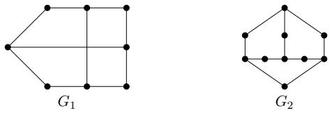
Reference graph

Works this paper leans on

34 extracted references · 31 canonical work pages

[33]

W. Zhen, D. Wong, S. Xu, Laplacian eigenvalue distribution and grith of graphs, Arxiv: 2504.15772v1

work page Pith review arXiv
[1]

Ahanjideh, S

M. Ahanjideh, S. Akbari, M.H. Fakharan, V. Trevisan, Laplacian eigenvalue distribution and graph parameters, Linear Algebra Appl. 632 (2022) 1–14

work page 2022
[2]

Akbari, M

S. Akbari, M. Alaeiyan, M. Darougheh, V. Trevisan, Classification of trees by Laplacian eigenvalue distribution and edge covering number, Linear Algebra Appl. 677 (2023) 221– 236

work page 2023
[3]

Anderson, T.D

W.N. Anderson, T.D. Morley, Eigenvalues of the Laplacian of a graph, Linear Multilin- ear Algebra 18 (1985) 141–145

work page 1985
[4]

Braga, V.M

R.O. Braga, V.M. Rodrigues, V. Trevisan, On the distribution of Laplacian eigenvalues of trees, Discrete Math. 313 (2013) 2382–2389

work page 2013
[5]

Brouwer, W

A. Brouwer, W. Haemers, Spectra of Graphs, Springer, New York, 2012

2012
[6]

Cardoso, D.P

D.M. Cardoso, D.P. Jacobs, V. Trevisan, Laplacian distribution and domination, Graphs Combin. 33 (2017) 1283–1295

work page 2017
[7]

J. Choi, S. Moon, S. Park, Classification of graphs by Laplacian eigenvalue distribution and independence number, Linear Multilinear Algebra 71 (2023) 2877–2893

work page 2023

Show all 34 references

[8]

J. Choi, S. O, J. Park, Z. Wang, Laplacian eigenvalue distribution of a graph with given independence number, Appl. Math. Comput. 448 (2023) 127943

2023
[9]

Das, The largest two Laplacian eigenvalues of a graph, Linear Multilinear Algebra 52(2004) 441–460

K.C. Das, The largest two Laplacian eigenvalues of a graph, Linear Multilinear Algebra 52(2004) 441–460

2004
[10]

Faria, Permanental roots and the star degree of a graph, Linear Algebra Appl

I. Faria, Permanental roots and the star degree of a graph, Linear Algebra Appl. 64 (1985) 255–265

1985
[11]

Fiedler, Algebraic connectivity of graphs, Czech

M. Fiedler, Algebraic connectivity of graphs, Czech. Math. J. 23 (98) (1973) 298–305

1973
[12]

Goldberg, G

F. Goldberg, G. Shapiro, The Merris index of a graph, Electron. J. Linear Algebra 10 (2003) 212–222. 17

2003
[13]

Grone, R

R. Grone, R. Merris, V.S. Sunder, The Laplacian spectrum of a graph, SIAM J. Matrix Anal. Appl. 11 (1990) 218–238

1990
[14]

Guo, On the second largest Laplacian eigenvalue of trees, Linear Algebra Appl

J. Guo, On the second largest Laplacian eigenvalue of trees, Linear Algebra Appl. 404 (2005) 251–261

2005
[15]

J. Guo, S. Tan, A relation between the matching number and Laplacian spectrum of a graph, Linear Algebra Appl. 325 (2001) 71–74

2001
[16]

J. Guo, X. Wu, J. Zhang, K. Fang, On the distribution of Laplacian eigenvalues of a graph, Acta Math. Sin. (Engl. Ser.) 27 (2011) 2259–2268

2011
[17]

J. Guo, J. Xue, R. Liu, Laplacian eigenvalue distribution, diameter and domination number of trees, Linear Multilinear Algebra 73 (2025) 763–775

2025
[18]

Hedetniemi, D.P

S.T. Hedetniemi, D.P. Jacobs, V. Trevisan, Domination number and Laplacian eigen- value distribution, European J. Combin. 53 (2016) 66–71

2016
[19]

Horn, C.R

R.A. Horn, C.R. Johnson, Matrix Analysis, Second ed., Cambridge Univ. Press, Cam- bridge, 2013

2013
[20]

Jacobs, E.R

D.P. Jacobs, E.R. Oliveira, V. Trevisan, Most Laplacian eigenvalues of a tree are small, J. Combin. Theory Ser. B 146 (2021) 1–33

2021
[21]

Kirkland, J.J

S.J. Kirkland, J.J. Molitierno, M. Neumann, B.L. Shader, On graphs with equal alge- braic and vertex connectivity, Linear Algebra Appl., 341 (2002) 45–56

2002
[22]

Merris, Laplacian matrices of graphs: a survey, Linear Algebra Appl

R. Merris, Laplacian matrices of graphs: a survey, Linear Algebra Appl. 197–198 (1994) 143–176

1994
[23]

Merris, The number of eigenvalues greater than two in the Laplacian spectrum of a graph, Portugal

R. Merris, The number of eigenvalues greater than two in the Laplacian spectrum of a graph, Portugal. Math. 48 (1991)345–349

1991
[24]

Mohar, The Laplacian spectrum of graphs, in: Y

M. Mohar, The Laplacian spectrum of graphs, in: Y. Alavi, G. Chartrand, O.R. Oeller- mann, A.J. Schwenk, Graph theory, Combinatorics, and Applications, Vol. 2, Wiley, New York, 1991, pp. 871–898

1991
[25]

Mohar, Laplace eigenvalues of graphs–a survey, Discrete Math

B. Mohar, Laplace eigenvalues of graphs–a survey, Discrete Math. 109 (1992) 171–183

1992
[26]

Pan, Sharp upper bounds for the Laplacian graph eigenvalues, Linear Algebra Appl

Y. Pan, Sharp upper bounds for the Laplacian graph eigenvalues, Linear Algebra Appl. 355 (2002) 287–295

2002
[27]

Sin, On the number of Laplacian eigenvalues of trees less than the average degree, Discrete Math

C. Sin, On the number of Laplacian eigenvalues of trees less than the average degree, Discrete Math. 343 (2020) 111986

2020
[28]

So, Commutativity and spectra of Hermitian matrices, Linear Algebra Appl

W. So, Commutativity and spectra of Hermitian matrices, Linear Algebra Appl. 212– 213 (1994) 121–129. 18

1994
[29]

L. Xu, B. Zhou, Proof of a conjecture on distribution of Laplacian eigenvalues and diameter, and beyond, Linear Algebra Appl. 678 (2023) 92–106

2023
[30]

L. Xu, B. Zhou, Laplacain eigenvalue distribution and diameter of graphs, Discrete Math. 347 (2024) 114001

2024
[31]

L. Xu, B. Zhou, Diameter vs. Laplacian eigenvalue distribution, Electron. J. Linear Algebra 40 (2024) 774–787

2024
[32]

Zhang, The Laplacian eigenvalues of graphs: a survey, Arxiv: 1111.2897v1

X. Zhang, The Laplacian eigenvalues of graphs: a survey, Arxiv: 1111.2897v1

arXiv
[34]

L. Zhou, B. Zhou, Z. Du, On the number of Laplacian eigenvalues of trees smaller than two, Taiwanese J. Math. 19 (2015) 65–75. 19

2015

Pith tools

Reviewed August 7, 2026 · model on record in the stance chip above.

[1] [33]

W. Zhen, D. Wong, S. Xu, Laplacian eigenvalue distribution and grith of graphs, Arxiv: 2504.15772v1

work page Pith review arXiv

[2] [1]

Ahanjideh, S

M. Ahanjideh, S. Akbari, M.H. Fakharan, V. Trevisan, Laplacian eigenvalue distribution and graph parameters, Linear Algebra Appl. 632 (2022) 1–14

work page 2022

[3] [2]

Akbari, M

S. Akbari, M. Alaeiyan, M. Darougheh, V. Trevisan, Classification of trees by Laplacian eigenvalue distribution and edge covering number, Linear Algebra Appl. 677 (2023) 221– 236

work page 2023

[4] [3]

Anderson, T.D

W.N. Anderson, T.D. Morley, Eigenvalues of the Laplacian of a graph, Linear Multilin- ear Algebra 18 (1985) 141–145

work page 1985

[5] [4]

Braga, V.M

R.O. Braga, V.M. Rodrigues, V. Trevisan, On the distribution of Laplacian eigenvalues of trees, Discrete Math. 313 (2013) 2382–2389

work page 2013

[6] [5]

Brouwer, W

A. Brouwer, W. Haemers, Spectra of Graphs, Springer, New York, 2012

2012

[7] [6]

Cardoso, D.P

D.M. Cardoso, D.P. Jacobs, V. Trevisan, Laplacian distribution and domination, Graphs Combin. 33 (2017) 1283–1295

work page 2017

[8] [7]

J. Choi, S. Moon, S. Park, Classification of graphs by Laplacian eigenvalue distribution and independence number, Linear Multilinear Algebra 71 (2023) 2877–2893

work page 2023