REVIEW 4 major objections 3 minor 8 references
A Positivity-Preserving Finite Element Framework for Accurate Dose Computation in Proton Therapy
T0 review · 4 major / 3 minor · reviewed 2026-08-07 · deepseek-v4-flash
Pith's one-line read A finite element method that keeps proton dose from going negative
desk verdict A useful numerical framework undermined by a reversed inequality and an unproven maximum principle; the positivity-preserving claims don't yet have the advertised theoretical support. read the letter →
The pith
A machine-rendered reading of the paper's core claim, the machinery that carries it, and where it could break.
The reading
What carries the argument
The load-bearing object is the convex set $K_h = \{v_h \in V : 0 \le v_h(x_i) \le \sup_{\Gamma_-} g\}$ of finite element functions whose nodal values respect the physical bounds, paired with the variational inequality: find $\psi_h^+ \in K_h$ such that $A(\psi_h^+, v_h - \psi_h^+) + B_h(\psi_h^+, v_h - \psi_h^+) \ge l(v_h - \psi_h^+)$ for all $v_h \in K_h$. This is a box-constrained version of the SUPG discretisation: the constraint enforces the nodal maximum principle exactly, while the SUPG stabilisation with $\delta_K \sim h_K / (2(|\omega| + |\Pi_0 S(E)|))$ provides the coercivity and continuity estimates that yield quasi-optimality and the stated error rates.
What would settle it
Solve the slab problem with zero inflow ($g=0$) and a positive interior source ($f=1$), with $\epsilon=0$. Along each characteristic the exact fluence grows with path length, so the true solution is positive in the interior while $\sup_{\Gamma_-} g = 0$ forces $K_h = \{0\}$; the variational inequality then returns zero fluence everywhere, and the $L^2$ error between numerical and exact fluence fails to vanish as $h \to 0$. This calculation directly tests whether the upper bound $\sup g$ is the correct constraint for the scheme.
Extended reading notes
Core claim
The central claim is that the positivity-preserving variational inequality scheme (21), posed on the convex feasible set $K_h = \{v_h \in V : 0 \le v_h(x_i) \le \sup_{\Gamma_-} g\}$ defined by nodal bounds, guarantees nonnegative fluence at every Lagrange node, and that the analogous variational inequality or elementwise constant projection for dose (72), (69) guarantees nonnegative dose. The paper states that this discrete nodal maximum principle is compatible with SUPG stabilisation, and that the combined scheme achieves optimal a priori convergence rates for fluence (Corollary 3.9) and for dose (Lemmas 4.2 and 4.5), with the rate improving to $O(h^{p+1/2})$ when angular diffusion is absent.
Load-bearing premise
The whole positivity guarantee rests on the claim that the true fluence always stays between zero and the maximum value of the incoming beam; if a physical situation such as an interior proton source pushes the fluence above that ceiling, the method silently clamps the solution and the promised accuracy has no support.
Editorial extensions
If this is right
- Standard SUPG solutions that exhibit spurious negative fluence or negative dose beyond the Bragg peak are replaced by solutions with no nodal undershoots or overshoots.
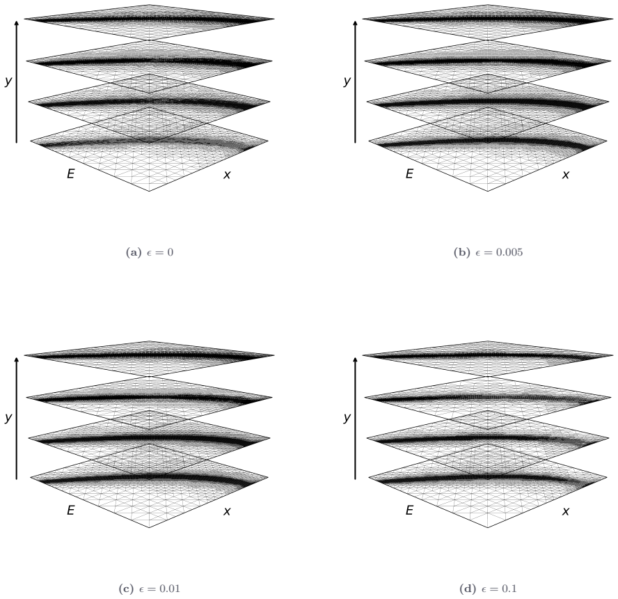
- The positivity-preserving scheme reproduces the Bragg peak position and magnitude with fewer degrees of freedom when driven by the residual-plus-jump adaptive indicator.
- The elementwise constant and variational inequality dose projections preserve nonnegativity, whereas the Galerkin L2 projection of dose does not.
- The same framework handles sharp material interfaces in layered heterogeneous media without post-processing or filtering.
- In the absence of angular diffusion, the a priori error rate improves to $O(h^{p+1/2})$, matching the hyperbolic character of the transport problem.
Reading between the lines
- If the continuous solution violates the upper bound $\sup_{\Gamma_-} g$ — for example with an interior source $f > 0$ — the variational inequality clamps the solution, and the paper's error estimates, which are proven for the unconstrained SUPG scheme, would not cover the clamped solution.
- For polynomial degree two or higher, nodal positivity does not imply pointwise positivity between nodes, so a dose evaluated at non-nodal points could still be negative even though all Lagrange nodes are nonnegative.
- Because $K_h$ is convex, the method could plug directly into treatment-planning optimisation as a convex constraint, making inverse planning with positivity constraints a natural next step.
- The same variational inequality projection can be applied to other energy-integrated observables such as LET-weighted dose, since the positivity argument only uses the positivity of $S$, $\rho$, and the quadrature weights.
Editorial analysis
A structured set of objections, weighed in public.
Referee Report
Summary. The paper proposes SUPG finite element discretisations for a deterministic proton transport model that combines streaming, continuous slowing-down via a Bragg--Kleeman stopping power, and angular diffusion through a Laplace--Beltrami operator. The main advertised innovation is a positivity-preserving variational inequality variant that restricts nodal values of the discrete fluence to the physical interval, and the paper claims optimal a priori error estimates for both fluence and dose, supported by numerical benchmarks. In my reading, the numerical experiments are suggestive, but the central theoretical arguments contain several load-bearing errors: the consistency proof is invalid for positive angular diffusion, the coercivity lemma contains a sign error and an integration-by-parts error, no error estimate is proved for the constrained variational inequality scheme, and the dose error bounds omit the fluence approximation error.
Significance. If the theoretical claims were valid, the paper would make a useful contribution to deterministic dose computation in proton therapy: positivity preservation on coarse meshes is practically important, and a deterministic alternative to Monte Carlo with guaranteed nonnegative fluence would be valuable for treatment planning. The paper also deserves credit for using reproducible tooling (Firedrake, PETSc, Netgen) and for presenting numerical comparisons against an analytic Bragg-peak solution and against the unconstrained SUPG method. However, the advertised optimal-rate theorems for the positivity-preserving scheme are not established by the proofs as written, and the errors are not merely cosmetic; they affect the main analytical contribution. The numerical sections alone do not compensate for the unsupported convergence claims.
major comments (4)
- [Section 3.5, Lemma 3.5 and Eq. (26)] The consistency proof is invalid for the angular diffusion case. From (8) and (17), the transport operator satisfies L(ψ) = f + εΔωψ, not L(ψ) = 0. Consequently the claim in (26) that the SUPG stabilisation term vanishes because the residual of L(ψ) is zero is false; the term Σ_K ∫_K δ_K L(ψ)L(v_h) does not vanish. The derivation of Galerkin orthogonality (49) and hence Theorem 3.8 and Corollary 3.9 depends on this cancellation, so the quasi-optimality result is not established for ε > 0. For ε = 0 the argument would go through, but the paper explicitly advertises the framework for the angular diffusion regime.
- [Section 3.6, Eqs. (35)-(39)] The coercivity proof contains a sign error and an integration-by-parts error. For S(E)=E^{1-p}/(αp), S' is increasing on [Emin,Emax], so S'(E) ≥ S'(Emin) = -μ. This gives ∫_Ω S' u_h^2 ≥ -μ ||u_h||^2, the reverse of the inequality printed in (37). Equivalently, -∫_Ω S' u_h^2 = ∫_Ω |S'| u_h^2 is at most μ||u_h||^2, so it cannot provide the +μ||u_h||^2 lower bound used in (39). Moreover, the integration by parts in (35) omits the +1/2∫_Ω S' u_h^2 term that appears when -∫_Ω ∂_E(Su_h)u_h is integrated by parts, so Eq. (36) is also algebraically inconsistent. A corrected calculation may yield a different coercivity constant, but Lemma 3.6 as stated is false, and the coercivity-based results depending on it are unsupported.
- [Section 3.3, Eq. (21), and Corollary 3.9] The abstract and introduction claim optimal a priori convergence rates for the positivity-preserving scheme, but no error estimate is proved for the constrained variational inequality solution ψ_h^+ defined in (21). Corollary 3.9 and Theorem 3.8 apply only to the unconstrained SUPG solution ψ_h of (19). For the variational inequality (21), the paper does not establish existence, uniqueness, a consistency inequality with the exact solution, or a quasi-optimality bound. Therefore the central claim that the positivity-preserving formulation achieves optimal rates is unproved. This is not a local technicality; it is the main theoretical contribution claimed in the abstract.
- [Section 4.2, Lemma 4.2, and Section 4.5, Lemma 4.5] The dose error bounds omit the fluence approximation error. In Lemma 4.2, Dh is defined from ψ_h, but the proof introduces D* using the exact ψ and then bounds ∥D*-Dh∥ as a spatial projection error with no reference to ∥ψ-ψ_h∥. The missing term is unavoidable: the difference between D* and Dh contains the factor S(E)/ρ(x) times ψ(x,ξ_q)-ψ_h(x,ξ_q), integrated against quadrature weights. Without including this term, the stated estimate (64) does not follow. The same omission occurs in Lemma 4.5, where (70) is asserted without accounting for ∥ψ-ψ_h∥ in the elementwise projection. These lemmas therefore do not provide the advertised dose error rates.
minor comments (3)
- [Section 5.1, Eq. (75)] The Gaussian inflow data uses ε in the denominator of the exponent, while δ is the parameter introduced for the energy spread; this appears to be a typo.
- [Section 5.2, Figure 9 caption] The caption contains an unresolved cross-reference to 'Figure ??', which should be corrected.
- [Section 3.9, proof of Corollary 3.9] The statement uses p for the polynomial degree and s for the Sobolev regularity, but the proof switches between k and p inconsistently; the notation should be unified.
Circularity Check
No significant circularity: positivity is transparently imposed by the feasible set, and the a priori error analysis is self-contained; self-citations are contextual, not load-bearing.
full rationale
The paper's central derivation chain is not circular. The positivity-preserving property is obtained by defining the discrete feasible set K_h = {v_h : v_h(x_i) ∈ [0, sup_Γ- g]} (Eq. 20) and then solving the variational inequality (21) over K_h; the paper states 'By construction, ψ_h+ ∈ K_h satisfies a nodal analogue of the maximum principle.' Thus the nonnegativity guarantee is an explicit imposed constraint, not a quantity fitted from data nor a prediction derived from a different input. The a priori error claims (Theorem 3.8, Corollary 3.9, Lemmas 4.2 and 4.5) are derived from consistency, coercivity, continuity, interpolation and quadrature estimates within the paper; they do not reuse the target error as an input, and no parameter is fitted to make the rates hold in the analysis. Self-citations ([Ash+25], [AHP25], [ABP24], [Bar+24]) supply the underlying transport model and the variational-inequality framework, but they are not used as a uniqueness theorem or to exclude alternatives, and the paper's mathematical estimates do not reduce to those citations. Empirical parameters (α, p) are taken from the literature (Bragg–Kleeman, Bortfeld), so no fitted input is relabelled as a prediction. The numerical benchmark in Sec. 5.1 compares against the exact solution of the same PDE, which is code verification rather than independent physical validation, but this is not a circular reduction of the paper's claims. Separate correctness concerns—e.g. the apparent sign of Eq. (37) (since S' is increasing, ∫S'u² ≥ -µ||u||², not ≤, so the coercivity lower bound (39) is not established) and the absence of an error estimate for the constrained solution of (21)—are gaps in proof, not circularity.
Assumptions & free parameters
free parameters (1)
- δK (SUPG stabilization parameter) =
h_K/(2(|ω| + |Π0 S(E)|))
assumptions (4)
- ad hoc to paper Continuous solution satisfies the maximum principle 0≤ψ≤sup_{Γ-}g (Remark 2.8).
- domain assumption Homogeneous Neumann condition ∇ωψ·nx=0 on Γ⊥(ω) (Eq 14, Remark 2.5).
- standard math Regularity ψ∈H^{s+1}(Ω) for the interpolation error estimates.
- ad hoc to paper The bilinear form A+B is coercive on V with the constant μ=-S'(Emin) (Lemma 3.6).
Cite this review
Pith. "Pith review of A Positivity-Preserving Finite Element Framework for Accurate Dose Computation in Proton Therapy." pith.science (2026). https://pith.science/paper/66TSM5EQ
@misc{pith2026250601105,
  author       = {Pith},
  title        = {Pith review of: A Positivity-Preserving Finite Element Framework for Accurate Dose Computation in Proton Therapy},
  year         = {2026},
  howpublished = {\url{https://pith.science/paper/66TSM5EQ}},
  note         = {Machine review of arXiv:2506.01105}
}
read the original abstract
We present a stabilised finite element method for modelling proton transport in tissue, incorporating both inelastic energy loss and elastic angular scattering. A key innovation is a positivity-preserving formulation that guarantees non-negative fluence and dose, even on coarse meshes. This enables reliable computation of clinically relevant quantities for treatment planning. We derive a priori error estimates demonstrating optimal convergence rates and validate the method through numerical benchmarks. The proposed framework provides a robust, accurate and efficient tool for advancing proton beam therapy.
Figures


Figures from the paper (8 more)



Reference graph
Works this paper leans on
-
[1]
A nodally bound-preserving finite element method for hyperbolic convection-reaction problems
[ABP24] A. Amiri, G. R. Barrenechea, and T. Pryer. “A nodally bound-preserving finite element method for reaction–convection–diffusion equations”. In: Mathematical Models and Methods in Applied Sciences 34.08 (2024), pp. 1533–1565. [AHP25] B. S. Ashby, A. Hamdan, and T. Pryer. “A nodally bound-preserving finite element method for hyperbolic convection-rea...
work page Pith review arXiv 2024
-
[52]
A fast Monte Carlo code for proton transport in radiation therapy based on MCNPX
[JS14] K. Jabbari and J. Seuntjens. “A fast Monte Carlo code for proton transport in radiation therapy based on MCNPX”. In: Journal of Medical Physics 39.3 (2014), pp. 156–163. [LGA03] A. J. Lomax, M. Goitein, and J. Adams. “Intensity modulation in radiotherapy: photons versus protons in the paranasal sinus”. In: Radiotherapy and Oncology 66.1 (Jan. 2003)...
-
[2004]
[Geo21] E. H. Georgoulis. “Hypocoercivity-compatible finite element methods for the long-time com- putation of Kolmogorov’s equation”. In: SIAM Journal on Numerical Analysis 59.1 (2021), pp. 173–194. [Ham+23] D. A. Ham et al. Firedrake User Manual . First edition. Imperial College London et al. May
work page 2021
-
[2006]
A Deterministic Dynamical Low-rank Approach for Charged Particle Transport
[Sal13] F. Salvat. “A generic algorithm for Monte Carlo simulation of proton transport”. In: Nuclear Instruments and Methods in Physics Research Section B: Beam Interactions with Materials and Atoms 316 (2013), pp. 144–159. [Sta+24] P. Stammer et al. “A Deterministic Dynamical Low-rank Approach for Charged Particle Trans- port”. In: arXiv preprint arXiv:2...
work page Pith review arXiv 2013
-
[2022]
Optimal control of a kinetic equation
[PPT24] A. Pim, T. Pryer, and A. Trenam. “Optimal control of a kinetic equation”. In: arXiv preprint arXiv:2412.10747 (2024). [PZ17] A. Porretta and E. Zuazua. “Numerical hypocoercivity for the Kolmogorov equation”. In: Math- ematics of Computation 86.303 (2017), pp. 97–119. [RHH23] T. J. Radley, P. Houston, and M. E. Hubbard. “Quadrature-free polytopic d...
work page Pith review arXiv 2024
-
[2023]
doi: 10.25561/104839. [HHR24] P. Houston, M. E. Hubbard, and T. J. Radley. “Iterative solution methods for high-order/hp– DGFEM approximation of the linear Boltzmann transport equation”. In: Computers & Mathe- matics with Applications 166 (2024), pp. 37–49. [Hou+24] P. Houston et al. “Efficient high-order space-angle-energy polytopic discontinuous Galerki...
doi:10.25561/104839 2024
-
[2301]
The Royal Society. 2024, p. 20230836. [Cro+25] A. Crossley et al. “Jump stochastic differential equations for the characterization of the Bragg peak in proton beam radiotherapy”. In: Proceedings of the Royal Society A 481.2310 (2025), p. 20240687. [DMS13] A. Dedner, P. Madhavan, and B. Stinner. “Analysis of the discontinuous Galerkin method for elliptic p...
work page 2025
-
[7359]
Cycle-Free Polytopal Mesh Sweeping for Boltzmann Transport
doi: 10.21105/joss.07359. [BK05] W. H. Bragg and R. Kleeman. “XXXIX. On the α particles of radium, and their loss of range in passing through various atoms and molecules”. In: The London, Edinburgh, and Dublin Philo- sophical Magazine and Journal of Science 10.57 (1905), pp. 318–340. 20 [Bor97] T. Bortfeld. “An analytical approximation of the Bragg curve ...
work page Pith review arXiv 1905
Reviewed August 7, 2026 · model on record in the stance chip above.
Discussion (0). Sign in to comment.